Combined ranking from multiple workbooks

dartistik

New Member
Joined
May 22, 2017
Messages
16
Hello all,

Last year I posted a question on here:

https://www.mrexcel.com/forum/excel...ng-automatically-after-entering-new-data.html

and in a matter of a couple of weeks I had a brilliant solution to my problem, thanks to a user called @B___P!

I now have another project in mind, and I could sure use some more help...

Once again I don't know if it is even possible to do what I would like, but here goes.


We currently have 22 divisions in our darts league pyramid in Denmark, and I would like to do a combined ranking of all the players across all divisions.

I have tried and tested how I want the ranking to work, but manually making a list of ~4,000 players and updating it every time they have played would be an impossible task. I need some automation.


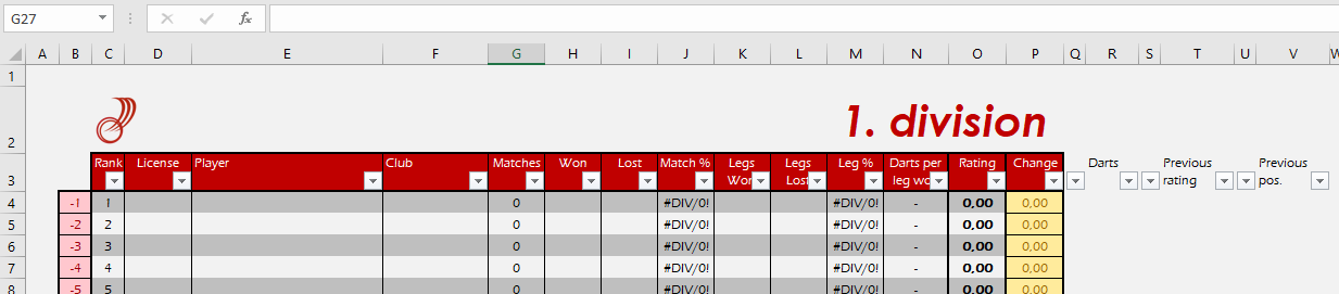
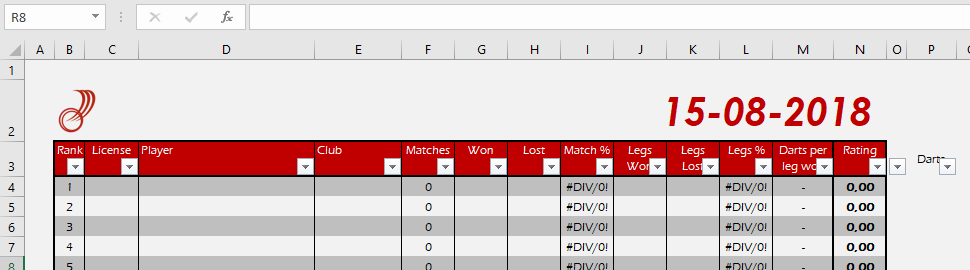
First of all, I need to make the list of all the players in 22 specific workbooks (one for each division):

- Scan the 22 workbooks for players by their unique license number (column D in the sheet named 'Samlet rangliste' in all the workbooks)
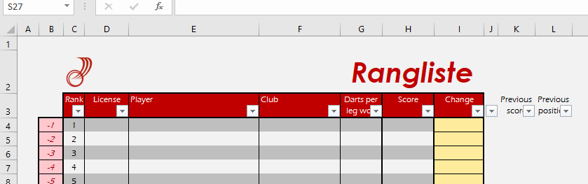
- List all players in another workbook called 'Rangliste' with the following information:

2805pqo.jpg

a) License (column D in 'Samlet rangliste' in all the workbooks) in column D
b) Name (column E in 'Samlet rangliste' in all the workbooks) in column E
c) Club (column F in 'Samlet rangliste' in all the workbooks) in column F
d) Score in column G​

- The 'Score' should be calculated in the following way:


a) If the player has only played in one division (license number only found in one workbook) it is fairly easy:​
The player's rating (column O in the sheet 'Samlet rangliste') x The average rating for the division (cell Y7 in the sheet 'Samlet rangliste')​

b) If the player has played in several divisions (license number found in multiple workbooks):
As above, but as a percentage of the total number of legs played in each division, for example:

Player A has played 10 legs in 1. division (column K+L in the sheet 'Samlet rangliste' in the workbook '1. division')
Player A has played 20 legs in 2. division Vest (column K+L in the sheet 'Samlet rangliste' in the workbook '2. division Vest')
He has then played 30 legs in total (columns K+L in 'Samlet rangliste' in both workbooks)


It should then be (10/30) x his rating in 1. division (column O in 'Samlet rangliste' in the workbook '1. division') x the average rating for that division (cell Y7) + (20/30) x his rating in 2. division Vest (column O in 'Samlet rangliste' in the workbook '2. division Vest') x the average rating for that division (cell Y7)


And so forth for all players who have played in multiple divisions (some may have played in more than two different divisions as well).​


Once the initial list has been built, I need the option to update the list every time the players have played in matches:

- Scan the 22 workbooks for license numbers and update the existing numbers correspondingly
- Add any new players not already in the list to the list using the same method as above, also adding a "-" in column J and K for the new players


Right, if anyone has even bothered to read that massive chunk of text, I'd be happy to send any info needed to anyone willing to give it a shot. I don't know if I explained it well enough or if it is in any way doable, but if it isn't then I'll at least know that.


Please don't hesitate to get in touch with any comments and I'd be most grateful! :rolleyes:
 
I'm at a bit of a loss, why do you need a formula in column H, when you can have the macro calculate whatever you want there? The first line starting with Licenses(r, 6) puts in what you want if there's no change, the next line starting with Licenses(r, 6) calculates the difference (if any). We could also add a bit of code to put something different there if it's a newly added player.

If you still want a formula, you can enter it like this:

Code:
Licenses(r, 6) = "=IF(RC[-1]<50,"""",""-"")"
I'd recommend the R1C1 style of cell reference to avoid having to calculate rows and columns.
 
Last edited:
Upvote 0

Excel Facts

Format cells as time
Select range and press Ctrl+Shift+2 to format cells as time. (Shift 2 is the @ sign).
Hi Eric,

My apologies - I'm not great with Excel, so I must have misunderstood you. If the macro can calculate what I want there, then of course there's no problem at all :)

The column is used to show the difference in the players's score after each update, so here's the formula that's in there now:

Code:
=IFERROR((ROUND(G4;2)-(ROUND(J4;2)));"NEW")

If the macro can just do the same, that would be great :)
 
Upvote 0
Yes, the macro can do that:

Rich (BB code):
Public Sub RankScores()
Dim MyPath As String, MyName As String, Status As String
Dim MyRow As Long, r As Long, i As Long, lnum As Long, Dict As Object
Dim Licenses(1 To 20000, 1 To 9), wktab As Variant, avg As Double, ix As Long, lr As Long
Dim L2() As Variant

' Initialization
    MyPath = "C:\Users\eweeks\Documents\Excel\Students\"
    
    Set Dict = CreateObject("Scripting.Dictionary")
    
    MyName = Dir(MyPath & "*.xl*")
    MyRow = 0
    
    Application.ScreenUpdating = False
    
' Find all the matching files in this directory.  get the scores
    On Error GoTo CloseIt:
    Do While MyName <> ""
        Workbooks.Open Filename:=MyPath & MyName
        Sheets("Samlet rangliste").Select
        avg = Range("Y7").Value
        wktab = Range("A1").Resize(Cells(Rows.Count, "D").End(xlUp).Row, 15).Value
        savmr = MyRow
        For r = 4 To UBound(wktab)
            lnum = wktab(r, 4)
            If Not Dict.exists(lnum) Then
                MyRow = MyRow + 1
                Dict.Add lnum, MyRow
                ix = MyRow
                Licenses(ix, 1) = ix
                Licenses(ix, 2) = lnum
                Licenses(ix, 3) = wktab(r, 5)
                Licenses(ix, 4) = wktab(r, 6)
            Else
                ix = Dict(lnum)
            End If
            Licenses(ix, 6) = Licenses(ix, 6) + wktab(r, 11) + wktab(r, 12)
            Licenses(ix, 5) = Licenses(ix, 5) + avg * (wktab(r, 11) + wktab(r, 12)) * wktab(r, 15)
        Next r
NextFile:
        ActiveWorkbook.Close savechanges:=False
        MyName = Dir()
    Loop


' Finalize scores, get previous scores


    On Error Resume Next
    lr = Cells(Rows.Count, "D").End(xlUp).Row
    wktab = Range("D4:G" & lr).Value
    ReDim L2(1 To MyRow, 1 To 9)
    For r = 1 To MyRow
        Licenses(r, 5) = Licenses(r, 5) / Licenses(r, 6)
        Licenses(r, 6) = "New"
        Licenses(r, 8) = "-"
        Licenses(r, 9) = "-"
        For i = 1 To UBound(wktab)
            If wktab(i, 1) = Licenses(r, 2) Then
                Licenses(r, 6) = "No change"
                If Licenses(r, 5) <> wktab(i, 4) Then
                    Licenses(r, 6) = WorksheetFunction.Round(Licenses(r, 5) - wktab(i, 4), 2)
                End If
                Licenses(r, 8) = wktab(i, 4)
                Licenses(r, 9) = i
                Exit For
            End If
        Next i
        For i = 1 To 9
            L2(r, i) = Licenses(r, i)
        Next i
    Next r
    
    Range("C4").Resize(UBound(L2), UBound(L2, 2)) = L2
    
' Sort the scores
    With ActiveSheet.Sort
        .SortFields.Clear
        .SortFields.Add Key:=Range("G4"), Order:=xlDescending
        .SetRange Range("D4:K" & UBound(L2) + 3)    ' The 3 means 3 rows before the first data row
        .Apply
    End With
        
' finalization
    Application.ScreenUpdating = True
    Exit Sub
    
CloseIt:
    Resume NextFile:


End Sub
The first red line will be what shows up in that column for a new player. The next red line is for an existing player with no score change, and the last red line calculates the change, if any.

I also found one minor glitch with the sort that I fixed.
 
Upvote 0
Hi Eric,

Excellent stuff, this is getting very close to being what I hoped for!

One question - some players change clubs mid-season, so may be listed at one club in one division and at another club in another division (but of course with the same unique license number). How will that affect the player listing here? Will it just list the player with the first club name found when scanning the target worksheets?
 
Upvote 0
Exactly. The first time the macro encounters an ID number, it saves the club name. When it encounters the ID in another workbook, it just updates the numbers needed to calculate the rating. When it gets to the point of updating the summary workbook, again it just searches for the ID to find the previous rating, so the club name will be what it found from the first workbook. So to be sure to get the current club name, you'll need to change it in all of the source workbooks.
 
Upvote 0
Great, thank you. I think this should be ready for putting out there!

Once I get this going, there's bound to be people who want something changed or added, so if they make any requests I deem sensible I might pop in here and bug you again at some point ;)

Thank you once again for your work!
 
Upvote 0
Hi @Eric W,

First of all, I'd like to say thank you once again for the work you did for me last year - it worked like a charm throughout the season!

Now, during the last year I have updated the layout of my workbooks to make it look a bit better, and this included formatting the tables as actual tables in the workbooks. This has naturally caused both the macro you made for me and the one @B___P made for me in this thread to not work as intended anymore.

Would it by any chance be possible to adjust the macros so they work with tables? Here are a few screenshots of what the workbooks look like now:

CQL1G0f
Unavngivet.png


This is the target sheet in the workbook from my first thread. Column B is not a table, Column C is a table by itself so the rank doesn't switch around when sorting, and Column D to V is the main table. So when the results are added from the other sheet (see screenshot below), the data should be updated in the same way as before for already existing players, and for new players it should add a row in Column B, add a table row in Column C and add table rows for the main table and insert the data in the new row.

Unavngivet.png


This is the sheet where the data from each round is entered (I make a new sheet for each date). The data from this should be collated into the aforementioned sheet. As before, Column B is a table by itself and Column C to P is the main table with the data.

And finally, below is a screenshot of what the sheet from this thread looks like now:

Unavngivet.png


Column C is once again a table by itself, while Column D to L is the table with the data. As you can see, I have added a 'Darts per leg won' column (Column G), as this has been requested by many of the players following this ranking. If possible, it would be great if the macro could gather the data for this column by going through the target workbooks like before, adding all numbers in the column 'Darts' (Column R in the sheet Samlet rangliste) for a specific license number, and dividing it by the summed number of the column 'Legs won' (Column K in the sheet Samlet rangliste), so that way we get the average number of darts used per leg won across all the leagues the specific player has played in.

If any of the posters that have helped me before are still active, any help would be much appreciated!
 
Upvote 0
Hi, I am still active. The problem is that this appears to require a fair bit of time to work on. Compounding the problem is the fact that my PC crashed last year, and I lost the test files I had. Recreating those would be time-consuming too. In any event, I'd probably need to see copies of your new workbooks anyway to see the table names and other changes. I'm pretty busy right now, so I may not be able to help this time around. You might want to open a new thread so that others can see it and maybe offer to help. By all means post the existing code so they can just modify it.

Good luck!
 
Upvote 0
Hi Eric,

Thanks for your reply - and sorry to hear about your PC crash and subsequent data loss! If at any point you do get some more time on your hands, I'd be happy to send you the workbooks needed.

I'll try to start a new thread in the coming days and see if anyone else is able to help :)
 
Upvote 0

Forum statistics

Threads
1,214,653
Messages
6,120,751
Members
448,989
Latest member
mariah3

We've detected that you are using an adblocker.

We have a great community of people providing Excel help here, but the hosting costs are enormous. You can help keep this site running by allowing ads on MrExcel.com.
Allow Ads at MrExcel

Which adblocker are you using?

Disable AdBlock

Follow these easy steps to disable AdBlock

1)Click on the icon in the browser’s toolbar.
2)Click on the icon in the browser’s toolbar.
2)Click on the "Pause on this site" option.
Go back

Disable AdBlock Plus

Follow these easy steps to disable AdBlock Plus

1)Click on the icon in the browser’s toolbar.
2)Click on the toggle to disable it for "mrexcel.com".
Go back

Disable uBlock Origin

Follow these easy steps to disable uBlock Origin

1)Click on the icon in the browser’s toolbar.
2)Click on the "Power" button.
3)Click on the "Refresh" button.
Go back

Disable uBlock

Follow these easy steps to disable uBlock

1)Click on the icon in the browser’s toolbar.
2)Click on the "Power" button.
3)Click on the "Refresh" button.
Go back
Back
Top