Hi,
Ive been working on a a dynamic INDEX / MATCH, which I've sovled. How ever the values I'm returning on not always unique, and I want to lookup other values from the same column/row.
<!--[if !mso]><style>v\:* {behavior:url(#default#VML);}o\:* {behavior:url(#default#VML);}x\:* {behavior:url(#default#VML);}.shape {behavior:url(#default#VML);}</style><![endif]--><style><!--table {mso-displayed-decimal-separator:"\."; mso-displayed-thousand-separator:"\,";}@page {margin:.75in .7in .75in .7in; mso-header-margin:.3in; mso-footer-margin:.3in;}td {padding:0px; mso-ignore adding; color:black; font-size:12.0pt; font-weight:400; font-style:normal; text-decoration:none; font-family:Calibri, sans-serif; mso-font-charset:0; mso-number-format:General; text-align:general; vertical-align:bottom; border:none; mso-background-source:auto; mso-pattern:auto; mso-protection:locked visible; white-space:nowrap; mso-rotate:0;}.xl63 {font-size:10.0pt; font-family:Arial, sans-serif; mso-font-charset:0;}.xl64 {font-size:8.0pt; font-weight:700; font-family:Arial; mso-generic-font-family:auto; mso-font-charset:0;}.xl65 {mso-number-format:"Short Date";}--></style>
<!--StartFragment--> <colgroup><col width="87" span="9" style="width:65pt"> </colgroup><tbody>
<!--EndFragment--></tbody>
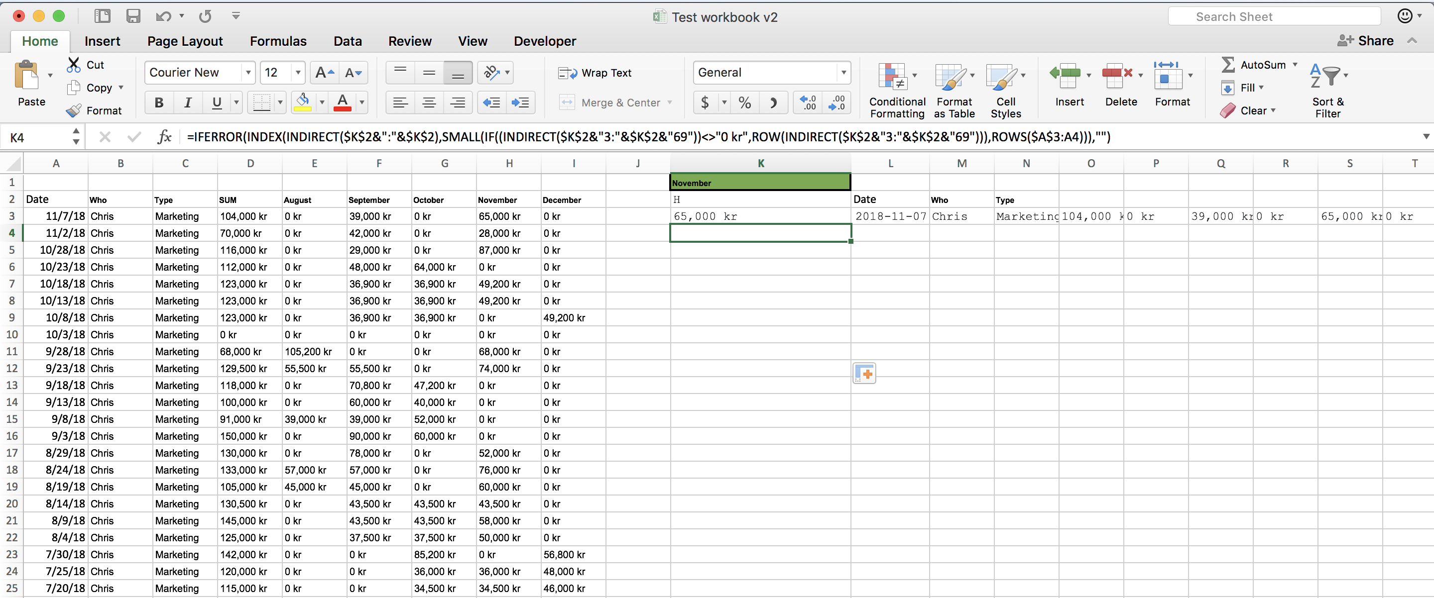
I have a data validation with the months which I've solved like this: =INDEX(Sheet1!$E$3:$I$1000,0,MATCH($K$1,Sheet1!$E$2:$I$2,0)) - so if I chose November from the dropdown list, I return all the values from the November column: <!--[if !mso]><style>v\:* {behavior:url(#default#VML);}o\:* {behavior:url(#default#VML);}x\:* {behavior:url(#default#VML);}.shape {behavior:url(#default#VML);}</style><![endif]--><style><!--table {mso-displayed-decimal-separator:"\."; mso-displayed-thousand-separator:"\,";}@page {margin:.75in .7in .75in .7in; mso-header-margin:.3in; mso-footer-margin:.3in;}td {padding:0px; mso-ignoreadding; color:black; font-size:12.0pt; font-weight:400; font-style:normal; text-decoration:none; font-family:Calibri, sans-serif; mso-font-charset:0; mso-number-format:General; text-align:general; vertical-align:bottom; border:none; mso-background-source:auto; mso-pattern:auto; mso-protection:locked visible; white-space:nowrap; mso-rotate:0;}.xl63 {color:black; font-size:10.0pt; font-family:Inconsolata; mso-generic-font-family:auto; mso-font-charset:0; background:yellow; mso-pattern:black none;}--></style>
<!--StartFragment--> <colgroup><col width="87" style="width:65pt"> </colgroup><tbody>
<!--EndFragment--></tbody>
Now, I would like to return the values from the other columns as well, for example for the first returned value in November I get "65,000kr", I would like to return the values from the Date, Who, Type columns as well.
<style><!--table {mso-displayed-decimal-separator:"\."; mso-displayed-thousand-separator:"\,";}@page {margin:.75in .7in .75in .7in; mso-header-margin:.3in; mso-footer-margin:.3in;}td {padding:0px; mso-ignoreadding; color:black; font-size:12.0pt; font-weight:400; font-style:normal; text-decoration:none; font-family:Calibri, sans-serif; mso-font-charset:0; mso-number-format:General; text-align:general; vertical-align:bottom; border:none; mso-background-source:auto; mso-pattern:auto; mso-protection:locked visible; white-space:nowrap; mso-rotate:0;}.xl63 {color:black; font-size:10.0pt; font-family:Inconsolata; mso-generic-font-family:auto; mso-font-charset:0; background:yellow; mso-pattern:black none;}--></style>
Ive been working on a a dynamic INDEX / MATCH, which I've sovled. How ever the values I'm returning on not always unique, and I want to lookup other values from the same column/row.
<!--[if !mso]><style>v\:* {behavior:url(#default#VML);}o\:* {behavior:url(#default#VML);}x\:* {behavior:url(#default#VML);}.shape {behavior:url(#default#VML);}</style><![endif]--><style><!--table {mso-displayed-decimal-separator:"\."; mso-displayed-thousand-separator:"\,";}@page {margin:.75in .7in .75in .7in; mso-header-margin:.3in; mso-footer-margin:.3in;}td {padding:0px; mso-ignore
adding; color:black; font-size:12.0pt; font-weight:400; font-style:normal; text-decoration:none; font-family:Calibri, sans-serif; mso-font-charset:0; mso-number-format:General; text-align:general; vertical-align:bottom; border:none; mso-background-source:auto; mso-pattern:auto; mso-protection:locked visible; white-space:nowrap; mso-rotate:0;}.xl63 {font-size:10.0pt; font-family:Arial, sans-serif; mso-font-charset:0;}.xl64 {font-size:8.0pt; font-weight:700; font-family:Arial; mso-generic-font-family:auto; mso-font-charset:0;}.xl65 {mso-number-format:"Short Date";}--></style>| Date | Who | Type | SUM | August | September | October | November | December |
| 11/6/18 | Chris | Marketing | 104,000 kr | 0 kr | 39,000 kr | 0 kr | 65,000 kr | 0 kr |
| 11/1/18 | Chris | Marketing | 70,000 kr | 0 kr | 42,000 kr | 0 kr | 28,000 kr | 0 kr |
| 10/27/18 | Chris | Marketing | 116,000 kr | 0 kr | 29,000 kr | 0 kr | 87,000 kr | 0 kr |
| 10/22/18 | Chris | Marketing | 112,000 kr | 0 kr | 48,000 kr | 64,000 kr | 0 kr | 0 kr |
| 10/17/18 | Chris | Marketing | 123,000 kr | 0 kr | 36,900 kr | 36,900 kr | 49,200 kr | 0 kr |
| 10/12/18 | Chris | Marketing | 123,000 kr | 0 kr | 36,900 kr | 36,900 kr | 49,200 kr | 0 kr |
| 10/7/18 | Chris | Marketing | 123,000 kr | 0 kr | 36,900 kr | 36,900 kr | 0 kr | 49,200 kr |
<!--StartFragment--> <colgroup><col width="87" span="9" style="width:65pt"> </colgroup><tbody>
<!--EndFragment--></tbody>
I have a data validation with the months which I've solved like this: =INDEX(Sheet1!$E$3:$I$1000,0,MATCH($K$1,Sheet1!$E$2:$I$2,0)) - so if I chose November from the dropdown list, I return all the values from the November column: <!--[if !mso]><style>v\:* {behavior:url(#default#VML);}o\:* {behavior:url(#default#VML);}x\:* {behavior:url(#default#VML);}.shape {behavior:url(#default#VML);}</style><![endif]--><style><!--table {mso-displayed-decimal-separator:"\."; mso-displayed-thousand-separator:"\,";}@page {margin:.75in .7in .75in .7in; mso-header-margin:.3in; mso-footer-margin:.3in;}td {padding:0px; mso-ignore
adding; color:black; font-size:12.0pt; font-weight:400; font-style:normal; text-decoration:none; font-family:Calibri, sans-serif; mso-font-charset:0; mso-number-format:General; text-align:general; vertical-align:bottom; border:none; mso-background-source:auto; mso-pattern:auto; mso-protection:locked visible; white-space:nowrap; mso-rotate:0;}.xl63 {color:black; font-size:10.0pt; font-family:Inconsolata; mso-generic-font-family:auto; mso-font-charset:0; background:yellow; mso-pattern:black none;}--></style>| 65,000 kr |
| 28,000 kr |
| 87,000 kr |
| 0 kr |
| 49,200 kr |
| 49,200 kr |
| 0 kr |
<!--StartFragment--> <colgroup><col width="87" style="width:65pt"> </colgroup><tbody>
<!--EndFragment--></tbody>
Now, I would like to return the values from the other columns as well, for example for the first returned value in November I get "65,000kr", I would like to return the values from the Date, Who, Type columns as well.
<style><!--table {mso-displayed-decimal-separator:"\."; mso-displayed-thousand-separator:"\,";}@page {margin:.75in .7in .75in .7in; mso-header-margin:.3in; mso-footer-margin:.3in;}td {padding:0px; mso-ignore
adding; color:black; font-size:12.0pt; font-weight:400; font-style:normal; text-decoration:none; font-family:Calibri, sans-serif; mso-font-charset:0; mso-number-format:General; text-align:general; vertical-align:bottom; border:none; mso-background-source:auto; mso-pattern:auto; mso-protection:locked visible; white-space:nowrap; mso-rotate:0;}.xl63 {color:black; font-size:10.0pt; font-family:Inconsolata; mso-generic-font-family:auto; mso-font-charset:0; background:yellow; mso-pattern:black none;}--></style>