Index , Vlookup Average Formula

[Sparda142]

Hello,

I am trouble creating a formula to go into Cells B2:I2, Im trying to have Excel say Find the Text "Scheduled Date" match the date below with a date in Row 1 and provide the information in Column M for Test 1 , Only Information from the Text "Scheduled Date to Subtotal" Belongs to Test 1. I have tried using a few IFS formula with combination of Vlookup but have failed.
Please help me create a formula that will do the job Excel Gods and have mercy on me! ray:

Column A

Column B

Column C

Column D

Column E

Column F

Column G

Column H

Column I

Column J

Column K

Column L

Column M

1

Test G

3/24

3/25

3/25

3/26

3/27

3/28

3/29

3/30

Total Average

N/A

N/A

2

Test 1

Test 1

N/A

3

Test 2

Schedule Date

N/A

Total Ad

4

Test 3

3/26

N/A

93.47%

5

Test 4

3/28

N/A

100%

6

Test 5

3/29

N/A

91.07&

7

Test 6

Subtotal:

N/A

94.85%

8

Test 2

N/A

9

Schedule Date

N/A

Total Ad

10

3/24

N/A

21.41%

11

3/25

N/A

67.25%

12

Subtotal:

N/A

13

Test 3

N/A

14

3/29

N/A

41.44%

15

3/30

N/A

99.99%

<tbody>
</tbody>

 

[kvsrinivasamurthy]

Does all the dates in Row 1 and column K are in date format.

 

[Mackers]

Hi

The easiest way I can think of without using a macro would be to add a helper column, say in N2:N15, that has the appropriate test written in every cell relating to information for that test.

In N2:

=IF(LEFT(K2,4)="Test",K2,N1)

And drag down. Then match on the combination of the date in K and the Test in N. Then, in B2:

=SUMIFS($M$2:$M$15,$K$2:$K$15,B$1,$N$2:$N$15,$A2)

Copy this across to I2 and then drag down to I7. This will only work if you have exactly one match and if your data in column M is numbers.

 

[Sparda142]

Yes. Originally Column K had the dates written as "Tuesday, 26 March 2019", I have use a "right" formula with a combination of "Datevalue" and copied over the text with a Date so the dates appear

 

[Sparda142]

This may not work due to "Test 1" is a Person and each has a different name length, Attached is the spread sheet i am working on. I;m trying to get the volume in column AB for the Individuals in column B by date.

[FONT=&quot]https://www.mediafire.com/file/o2i9h1bijyj12zb/Adherance_Template.xlsx/file[/FONT]

 

[sheetspread]

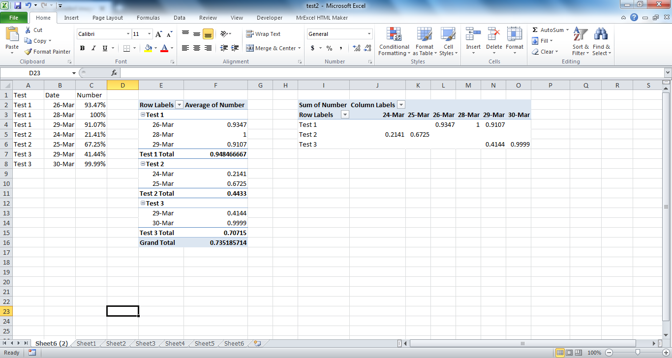
Without changing the data structure, we'd have to write an equally clunky formula. Much better is to neaten it up like:

Then you can pivot as desired.

Here's how to label each row:

Excel 2010
	A	B	C	D
1		N/A	N/A
2	Test 1	Test 1	N/A
3	Test 1	Schedule Date	N/A	Total Ad
4	Test 1	26-Mar	N/A	93.47%
5	Test 1	28-Mar	N/A	100%
6	Test 1	29-Mar	N/A	91.07%
7	Test 1	Subtotal:	N/A	94.85%
8	Test 2	Test 2	N/A
9	Test 2	Schedule Date	N/A	Total Ad
10	Test 2	24-Mar	N/A	21.41%
11	Test 2	25-Mar	N/A	67.25%
12	Test 2	Subtotal:	N/A
13	Test 3	Test 3	N/A
14	Test 3	29-Mar	N/A	41.44%
15	Test 3	30-Mar	N/A	99.99%
Sheet6

Cell Formulas
Range	Formula
A2	=IF(LEFT(B2,4)="Test",B2,A1)

then delete the extras either by sorting first or with F5-Goto-Special-Text

 

[Mackers]

If the consistent thing that indicates the next test is the "Subtotal:" cell, you could instead check for subtotals like this (in A8):

=IF(B7="Subtotal:",B8,A7)

 

[Sparda142]

So I have deleted a bunch of information that wasn't needed and am now here. Would a INDEX & Match with multiple criteria to make the Percent come up in cell b2 if A2 and B1 match?

	a	b	c	d	e	f	g	h	i
1		3/24	3/25	3/26	3/27	empty Column	NAME & Dates	Percent
2	Jacob						Jacob
3	Jill						3/24	100%
4	Scott						3/27	25%
5	Tim						Jill
6	Matt						3/25	30%
7	Howard						3/26	100%
8							3/27	99%
9							Scott
10							3/24	80%
11							3/27	75%
12							3/30	80%
13							Tim
							3/29	99%
							Matt
							3/28	63%

<tbody>
</tbody>

 

[sheetspread]

If you must........

Excel 2010
	A	B	C	D	E	F	G	H	I	J	K
1		24-Mar	25-Mar	26-Mar	27-Mar	28-Mar	29-Mar	30-Mar	empty Column	NAME & Dates	Percent
2	Jacob	100%	#N/A	#N/A	25%	#N/A	#N/A	#N/A		Jacob
3	Jill	#N/A	30%	100%	99%	#N/A	#N/A	#N/A		24-Mar	100%
4	Scott	80%	#N/A	#N/A	75%	#N/A	#N/A	80%		27-Mar	25%
5	Tim	#N/A	#N/A	#N/A	#N/A	#N/A	99%	#N/A		Jill
6	Matt	#N/A	#N/A	#N/A	#N/A	63%	#N/A	#N/A		25-Mar	30%
7	Howard	#N/A	#N/A	#N/A	#N/A	#N/A	#N/A	#N/A		26-Mar	100%
8										27-Mar	99%
9										Scott
10										24-Mar	80%
11										27-Mar	75%
12										30-Mar	80%
13										Tim
14										29-Mar	99%
15										Matt
16										28-Mar	63%
17										Howard
Sheet7

Cell Formulas
Range	Formula
B2	=VLOOKUP(B$1,OFFSET(INDEX($J$2:$J$17,MATCH($A2,$J$2:$J$17,0)),,,MATCH($A3,$J$2:$J$17,0)-MATCH($A2,$J$2:$J$17,0),2),2,0)

I might be able to post a slightly shorter version

 

[Sparda142]

The formula isn't working exactly as shown, I've attached a link to show. Row 2 b2 is coming up as 100% while Row 3 b3:h3 show #N/A


https://ibb.co/spTRY9Y