Highlight values that have triggered an IF / SUMIFS statement

ajnin

New Member
Joined
Apr 26, 2019
Messages
7
Office Version
  1. 2019
Platform
  1. Windows
Hello,

Is there a way to highlight values that have been used in a formula :confused:

Example formula
=(SUMIFS(All!$B:$B,All!$A:$A,">=1/1/2018",All!$A:$A,"<=31/1/2018",All!$C:$C,"shop1")+(SUMIFS(All!$B:$B,All!$A:$A,">=1/1/2018",All!$A:$A,"<=31/1/2018",All!$C:$C,"shop2")))*-1

My data looks like this
vznCZgz.png

DbWxkpc


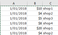
I would like to have all instances of shop1 and shop2 highlighted. As they are in the above formula. i would need to do this for a bunch of formulas all looking for different values.

Or if doing it in reverse is more easy, that would also work. Or any other way I can easy identify what in my data has not been captured by the if statements.

Thanks :)
 

Excel Facts

Formula for Yesterday
Name Manager, New Name. Yesterday =TODAY()-1. OK. Then, use =YESTERDAY in any cell. Tomorrow could be =TODAY()+1.
Re: How to Highlight values that have triggered an IF / SUMIFS statement

Hey, you could use Conditional Formatting to do this.

You'll have to make a rule for each SUMIFS statement I believe but it is possible. For example to highlight all of 3 columns that hold true under the first SUMIFS statement (shop1) then use this CF formula:
=AND($A1>=43101,$A1<=43131,$C1="shop1")
Here 43101 is the serial number of 01/01/2018 and 43131 the serial number of 31/01/2018.

Then make sure this applies to your A:C range that the data is in (=$A$1:$C$#) # being the last row

EDIT: If you want the dates more dynamic than serial number then you could use DATE(2018,1,1) and DATE(2018,31,1) instead of 43101 & 43131.
 
Last edited:
Upvote 0
Re: How to Highlight values that have triggered an IF / SUMIFS statement

Thanks for the advise. I will give this a go. Also thanks for the DATE(2018,1,1) tip :)

Hey, you could use Conditional Formatting to do this.

You'll have to make a rule for each SUMIFS statement I believe but it is possible. For example to highlight all of 3 columns that hold true under the first SUMIFS statement (shop1) then use this CF formula:
=AND($A1>=43101,$A1<=43131,$C1="shop1")
Here 43101 is the serial number of 01/01/2018 and 43131 the serial number of 31/01/2018.

Then make sure this applies to your A:C range that the data is in (=$A$1:$C$#) # being the last row

EDIT: If you want the dates more dynamic than serial number then you could use DATE(2018,1,1) and DATE(2018,31,1) instead of 43101 & 43131.
 
Upvote 0

Forum statistics

Threads
1,214,920
Messages
6,122,267
Members
449,075
Latest member
staticfluids

We've detected that you are using an adblocker.

We have a great community of people providing Excel help here, but the hosting costs are enormous. You can help keep this site running by allowing ads on MrExcel.com.
Allow Ads at MrExcel

Which adblocker are you using?

Disable AdBlock

Follow these easy steps to disable AdBlock

1)Click on the icon in the browser’s toolbar.
2)Click on the icon in the browser’s toolbar.
2)Click on the "Pause on this site" option.
Go back

Disable AdBlock Plus

Follow these easy steps to disable AdBlock Plus

1)Click on the icon in the browser’s toolbar.
2)Click on the toggle to disable it for "mrexcel.com".
Go back

Disable uBlock Origin

Follow these easy steps to disable uBlock Origin

1)Click on the icon in the browser’s toolbar.
2)Click on the "Power" button.
3)Click on the "Refresh" button.
Go back

Disable uBlock

Follow these easy steps to disable uBlock

1)Click on the icon in the browser’s toolbar.
2)Click on the "Power" button.
3)Click on the "Refresh" button.
Go back
Back
Top