Please see the imagine.
https://imgur.com/a/haW7m1x
I have a table of information.
you can seen cell C15 shows certification number is 2.
What formula should I use in cell C16 so it shows 123, 321, 111.
concatenate unique values only, based on criteria without macros?
How is it done?
Thank you in advance.
https://imgur.com/a/haW7m1x
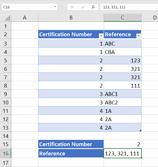
I have a table of information.
you can seen cell C15 shows certification number is 2.
What formula should I use in cell C16 so it shows 123, 321, 111.
concatenate unique values only, based on criteria without macros?
How is it done?
Thank you in advance.