Accrued Revenue Ageing Formula

[ryansm05]

Hi,

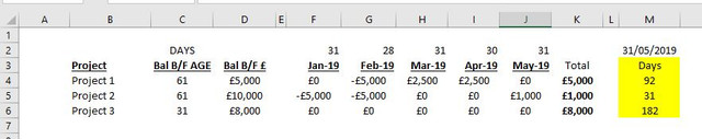
From the below, I need to work out the ageing of the balances. The figures in column M (highlighted yellow) are the values I'm looking to achieve, which incorporates the following:

1) The Bf balance in column C. For Project 1 this is 61 days for the £5,000.

2) The formula will understand that this balance was cleared for Project 1 in February (G4). Subsequently the ageing of Project 1 in Feb 19 reverts to 0.

3) The values in H4 and I4 (£2,500 x 2) are generated in Mar 19 and Apr 19 respectively, and therefore the ageing restarts.

4) At 31/05/2019 (M2) the ageing of Project 1 is 92 days. This is because the balance started to generate in H4 and has not yet been cleared.




I appreciate this is quite a complex request, so if anyone can help, it'd be much appreciated.

Cheers
Ryan

 

[steve the fish]

If you are going to put sample data on the forum please paste something we can copy paste straight into excel not a picture. Anyway lets take project 1. What happens if the brought forward balance is not cleared in full eg if they had only paid say 4000 in Feb? What is the answer required then?

 

[ryansm05]

If you are going to put sample data on the forum please paste something we can copy paste straight into excel not a picture. Anyway lets take project 1. What happens if the brought forward balance is not cleared in full eg if they had only paid say 4000 in Feb? What is the answer required then?

Apologies for that Steve.

In your example, since the balance is not cleared in full, I would want the ageing to include the BF figure. Do you think that’s possible?

Thanks!
Ryan

 

[steve the fish]

There must be something less intimidating but this works for your examples at least:

=IF(SUMPRODUCT(--(SIGN(F4:J4)=-1),-F4:J4)>=D4,SUM(INDEX($F$2:$J$2,MIN(IF(COLUMN(F4:J4)-COLUMN(F4)+1>MAX(IF(F4:J4<0,COLUMN(F4:J4)-COLUMN(F4)+1)),IF(F4:J4>0,COLUMN(F4:J4)-COLUMN(F4)+1)))):$J$2),SUM($F$2:$J$2,C4))

Requires CTRL-SHIFT-ENTER not just enter. Look for {} appearing around the formula if entered correctly.

 

[ryansm05]

Hi Steve,

thanks so much for this - the formula is icnredible!


However, although it work it works in almost every instance, there are a few examples where it doesn't which are highlighted red.
For example, Project 2 should be 151 + 61 as the balance has not yet been reduced to 0 at any point. It's the opposite with Project 7. It seems they're almost defaulting to the 151.

				31	28	31	30	31
Project		BF (days)	BF (£)	Jan 19	Feb 19	Mar 19	Apr 19	May 19	Jun 19	Jul 19	Aug 19	Sep 19	Oct 19	Nov 19	Dec 19		Total	Ageing (days)	Comments
Project 1		0	0	0	0	2000	3200	2600									7800	92	Correct
Project 2		61	16000	-7000	-4000	9000	-6903	-1126									5971	151	Incorrect: the ageing should be 212 (151 + 61) as the balance has not yet been reduced to 0
Project 3		0	0	0	0	0	0	23465									23465	31	Correct
Project 4		0	0	0	0	8000	0	0									8000	92	Correct
Project 5		0	0	0	7500	-2300	5000	-2850									7,350	151	Incorrect: the ageing should be 120 days as the balance has not yet been reduced to 0
Project 6		0	0	0	0	0	0	9185									9185	31	Correct
Project 7		91	21425	3740	-25165	3138	-57	0									3081	151	Incorrect: the ageing should be 92 days as the balance was reduced to 0 in Feb 19.
Project 8		31	8000	0	0	0	0	0									8000	182	Correct
Project 9		0	0	0	0	0	10000	21500									31500	61	Correct
Project 10		31	28388	-28388	0	4160	24227	0									28387	92	Correct
Totals

<tbody>
</tbody>

=IF(R7=0,0,IF(SUMPRODUCT(--(SIGN(E7:P7)=-1),-E7:P7)>=D7,SUM(INDEX($E$5:$P$5,MIN(IF(COLUMN(E7:P7)-COLUMN(E7)+1>MAX(IF(E7:P7<0,COLUMN(E7:P7)-COLUMN(E7)+1)),IF(E7:P7>0,COLUMN(E7:P7)-COLUMN(E7)+1)))):$P$5),SUM($E$5:$P$5,C7)))

Let me know if you have a work around?!

Thanks again,
Ryan

 

[ryansm05]

Hi Steve,

I've realised that probably wasn't helpful - so I've uploaded the file to DropBox: https://www.dropbox.com/s/u43rntfp1iwrbvr/Acc Rev Formula.xlsx?dl=0

Hope this is easier to follow!

Thanks
Ryan

 

[ryansm05]

Sorry to bump this - but if anyone else could help, it would be much appreciated (it almost very nearly works as needed).

Thanks!
Ryan