Stop looking in the first visible cell and return the value in the reference cell

thienan0701

New Member
Joined
Jun 21, 2019
Messages
4
Hi all,
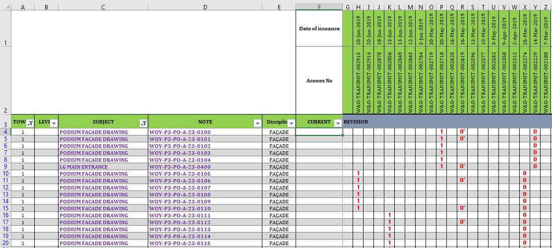
I want to stop searching in the first visible cell in the data range and return the result to the reference cell as the picrure shown below.
For example,
I want to input formula in Cell F4, my data range is G4-Z4, the result will return to the reference cell is P2.
Thank you all :biggrin:

dkyGIwF.png
 

Excel Facts

What did Pito Salas invent?
Pito Salas, working for Lotus, popularized what would become to be pivot tables. It was released as Lotus Improv in 1989.
Enter as an array formula (i.e. by pressing Ctrl+Shift+Enter) in cell F4:

Code:
= OFFSET( F4, , MATCH( TRUE, LEN( G4:Z4 ) > 0, 0 ) )
 
Upvote 0
Enter as an array formula (i.e. by pressing Ctrl+Shift+Enter) in cell F4:

Code:
= OFFSET( F4, , MATCH( TRUE, LEN( G4:Z4 ) > 0, 0 ) )

Thanks ParamRay.
The result I want to return is row 2, corresponds to the column which the result stop.
For example:
1. If I enter the formular on cell F4, the result is W&O-TRANSMIT-002718(on cell P)
2. Lock the result on row 2 so that I can array the formula down.
 
Upvote 0
Ok I understand. So just change F4 in my original formula with F$2. And remember to enter it using ctrl+shift+enter. Then you can drag the formula down.
 
Upvote 0
Ok I understand. So just change F4 in my original formula with F$2. And remember to enter it using ctrl+shift+enter. Then you can drag the formula down.

Thanks for your reply,
I’m sorry for the inconvenience, but I mean.
If I enter the formular on cell F4, the result is W&O-TRANSMIT-002718(on cell P2)
F10, the result is W&O-TRANSMIT-002915(on cell H2)
F16, the result is W&O-TRANSMIT-002856(on cell K2)
 
Upvote 0
Thanks for your reply,
I’m sorry for the inconvenience, but I mean.
If I enter the formular on cell F4, the result is W&O-TRANSMIT-002718(on cell P2)
F10, the result is W&O-TRANSMIT-002915(on cell H2)
F16, the result is W&O-TRANSMIT-002856(on cell K2)

Yes, I know. Enter the formula above (with the discussed adjustment) into cell F4 and drag down.
 
Upvote 0

Forum statistics

Threads
1,214,400
Messages
6,119,288
Members
448,885
Latest member
LokiSonic

We've detected that you are using an adblocker.

We have a great community of people providing Excel help here, but the hosting costs are enormous. You can help keep this site running by allowing ads on MrExcel.com.
Allow Ads at MrExcel

Which adblocker are you using?

Disable AdBlock

Follow these easy steps to disable AdBlock

1)Click on the icon in the browser’s toolbar.
2)Click on the icon in the browser’s toolbar.
2)Click on the "Pause on this site" option.
Go back

Disable AdBlock Plus

Follow these easy steps to disable AdBlock Plus

1)Click on the icon in the browser’s toolbar.
2)Click on the toggle to disable it for "mrexcel.com".
Go back

Disable uBlock Origin

Follow these easy steps to disable uBlock Origin

1)Click on the icon in the browser’s toolbar.
2)Click on the "Power" button.
3)Click on the "Refresh" button.
Go back

Disable uBlock

Follow these easy steps to disable uBlock

1)Click on the icon in the browser’s toolbar.
2)Click on the "Power" button.
3)Click on the "Refresh" button.
Go back
Back
Top