hi,
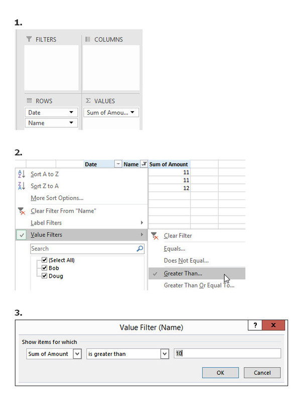
The simple filtering explained by Sandy is great. Hopefully that is sufficient for your requirements.
Below are some other ideas FYI.
One way with an existing pivot table is to add another field to the source data. Say "ShowIt".
Populate with a formula that links to the pivot table, something like
=GETPIVOTDATA(references to get the total you want to check against)>10
Now make a second pivot table & put the ShowIt field as a page field to filter for TRUE.
Refresh the first then the second pivot table if data changes.
More complex is if you want the result directly in a pivot table, and without adding an extra field to the data. This can be done by creating a dataset that already has the filtering.
Such as defining the dataset by, untested
Code:
SELECT A.[Date], A.Name, A.Amount
FROM YourDataName A
GROUP BY A.[Date], A.Name
HAVING SUM(A.Amount) > 10
This works in all versions of pivot tables, BTW. Detailed steps follow, or search for examples via Google.
When the source data has simple defined name "YourDataName". Such as select the data then CTRL-F3 & define the named range, or via the name box at top LHS.
Field name "Date" may be a problem - hopefully enclosing in brackets avoids issues.
Having saved the data file, safest for earlier Excel versions is to then have a new file when creating the pivot table.
So, CTRL-N for a new Excel file
ALT-D-P to start the pivot table wizard
external data source at the first stop then follow the wizard to the end choosing the option then to edit in MS Query.
Via the SQL button define the dataset as above, OK to enter & OK again if you get a message. See the results set.
Via the open door button exit MS Query & complete the pivot table.
Having created the pivot table on a worksheet, you can if you want move the entire worksheet to the same workbook as the data.
regards, Fazza
")


