Sum of unique values for conditional lookup

[drsgizmo]

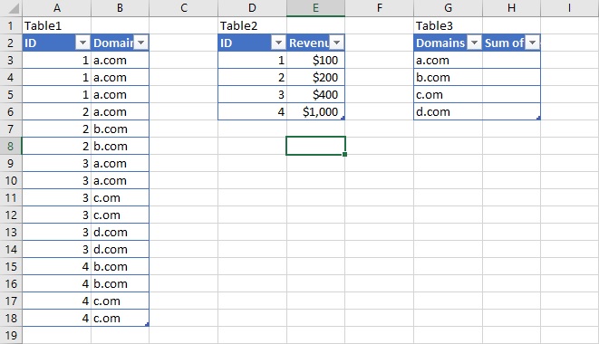
For this dataset, I'm trying to write a formula in Table3 that will sum the revenue amount (from Table2) of any ID that is associated with domain in Table1. The formula should first pull the list of unique IDs that are associated with the domain, so for 'a.com' it would create the array {1,2,3}. It would then find the revenue amount for each of those IDs, so {1,2,3} becomes {100,200,400}. It would then sum that array, in this case to arrive at $700. I've tried so far this

{=SUM(IF(COUNTIFS(Table1[Domains],$G$3,Table1[ID],$D$3:$D$6)>0,INDEX(Table2[Revenue], MATCH($D$3:$D$6, Table2[ID],0)),0))}

and

{=SUM(IF($B$3:$B$18=G3,VLOOKUP($A$3:$A$18,$D$3:$E$6,2,0),0))}

neither of which work. Any help is very appreciated.

 

[kweaver]

Where are the revenue numbers coming from? You don't show that in your post.

 

[drsgizmo]

So the revenue-ID relationship and the ID-domain relationship are hard-coded. The revenue-ID relationship is in Table2 above.

 

[drsgizmo]

To be clearer, for the Table3 cell adjacent to a.com, it would look in Table1 and find that there is at least one instance of IDs 1, 2, and 3 associated with a.com, but no instances of ID 4. For 1, 2, and 3, it would look in Table2 to find the associated revenue amounts, which are contained in cells E3, E4, and E5. It would then add E3+E4+E5 to find the revenue sum for a.com.

 

[Marcelo Branco]

Assuming the IDs are numbers, not Alphanumeric, maybe this

Array formula in H3 (Table3)
=SUM(SUMIF(Table2[ID],IF(FREQUENCY(IF(Table1[Domain]=[@Domain],Table1[ID]),Table1[ID]),Table1[ID]),Table2[Revenue]))
confirmed with Ctrl+Shift+Enter, not just Enter

Hope this helps

M.

 

[drsgizmo]

Works great! Thank you for your help. I'm having a little trouble figuring out how it works; if you have time for an explanation, that would be great. If not, no worries.

 

[Marcelo Branco]

You are welcome. Glad to help

The key part of the formula is
IF(FREQUENCY(IF(Table1[Domain]=[@Domain],Table1[ID]),Table1[ID]),Table1[ID])

It yields, in memory, an array of unique IDs that meet the criteria (G3) and FALSE values - something like this (FALSO in Portuguese = FALSE in English)

1​

FALSO​

FALSO​

2​

FALSO​

FALSO​

3​

FALSO​

FALSO​

FALSO​

FALSO​

FALSO​

FALSO​

FALSO​

FALSO​

FALSO​

FALSO​

<tbody>
</tbody>

Then SUMIF generates another array that is passed to the SUM function

To see what the formula does, step by step, try
Formulas > Evaluate Formula

M.

 

[drsgizmo]

Got it. Thanks very much for the explanation.

 

[Marcelo Branco]

You are welcome. Thanks for the feedback.

M.

 

[drsgizmo]

One last question for you: is this possible with an open or partial match? So if, for example, the value under "domains" in Table3 said "a." and we wanted it to catch instances of "a.com" and "b.a.com"? I don't think just substituting IF(Table1[Domain]="*"&[@Domain]&"*" will work, will it?