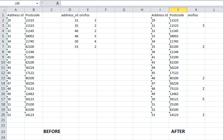
Put a value to a cell only if two values of two other columns are the same

antstyl

New Member
Joined
Mar 1, 2015
Messages
14
Hello everyone,
i tried to search and find what I am looking for but with no success probably because I cannot describe it very well. I will try to explain what I need with a picture.
Thanks for your assistance in advance.


yVz36Q0
nN14kHN.png
 
Hey,

If you manually overwrite the values in column J does the formula work? It looks like the numbers in J aren't being stored as numbers - numbers are right-aligned.

Otherwise try this formula that adapts column J to a numerical value and then evaluates it:

L2:
Code:
IF(SUMPRODUCT((VALUE(J2)=$F$2:$F$21)*(ISNUMBER($G$2:$G$21)))=0,"",INDEX($F$2:$G$21,MATCH(VALUE(J2),$F$2:$F$21,FALSE),2))
 
Last edited:
Upvote 0

Excel Facts

Which Excel functions can ignore hidden rows?
The SUBTOTAL and AGGREGATE functions ignore hidden rows. AGGREGATE can also exclude error cells and more.
thanks, it works great with this second formula!!!

Is there any way to be able to read also text and copy it to the new cell?
I think this is a totally different formula because of not being numbers and I dont want to bother you anymore if it is something complicated.
 
Upvote 0
thanks, it works great with this second formula!!!

Is there any way to be able to read also text and copy it to the new cell?
I think this is a totally different formula because of not being numbers and I dont want to bother you anymore if it is something complicated.

What exactly do you mean by the bit in red? To read the greek letters and copy it across?
 
Upvote 0
In the file that I had attached previously as a sample, there is a column "orofos" which was the column that I wanted to be copied next to the column "company_id" if the numbers in "address_id" were the same.
If the column "orofos" contains numbers (as it was in the sample) it does it perfect. But is there a way the same to be done if "orofos" contains also text?
 
Upvote 0
OK try this in cell M2:

Code:
IF(SUMPRODUCT((VALUE($J2)=$F$2:$F$21)*(ISTEXT($G$2:$G$21)))=0,"",INDEX($F$2:$G$21,MATCH(VALUE($J2),$F$2:$F$21,FALSE),2))

Drag it down the M column - it should return "NULL" where the address_id matches (as that is the text value in orofos in this sample data) - it will change according to column G.
 
Upvote 0
It works as it should be! thanks and those two formulas are very useful for me and hopefully for others as it combines columns from two different exports that I had.

Would you blast on me ( :p ) if I asked if there is any chance to make this work simultaneously? I mean being able to read and copy both cases, if it is number or text..
 
Upvote 0
No problem, I believe the following should work:

Try this in N2 to start and drag down (to see if it works for you) if yes, then you can replace L & M formulae with this one.

N2:
Code:
IF(SUMPRODUCT((VALUE($J2)=$F$2:$F$21)*(IF(ISTEXT($G$2:$G$21),ISTEXT($G$2:$G$21),ISNUMBER($G$2:$G$21))))=0,"",INDEX($F$2:$G$21,MATCH(VALUE($J2),$F$2:$F$21,FALSE),2))
 
Upvote 0
this worked perfect!!
It did exactly what I needed to....
Just a quick..was it too special this one? I mean it seems to me very common as a case, someone to need this in excel, but I couldn't find anywhere any guidance on this.

Once more thank you very much for your help and your willing to spend your valuable time on answering all these questions!!
 
Upvote 0

Forum statistics

Threads
1,214,515
Messages
6,119,973
Members
448,933
Latest member
Bluedbw

We've detected that you are using an adblocker.

We have a great community of people providing Excel help here, but the hosting costs are enormous. You can help keep this site running by allowing ads on MrExcel.com.
Allow Ads at MrExcel

Which adblocker are you using?

Disable AdBlock

Follow these easy steps to disable AdBlock

1)Click on the icon in the browser’s toolbar.
2)Click on the icon in the browser’s toolbar.
2)Click on the "Pause on this site" option.
Go back

Disable AdBlock Plus

Follow these easy steps to disable AdBlock Plus

1)Click on the icon in the browser’s toolbar.
2)Click on the toggle to disable it for "mrexcel.com".
Go back

Disable uBlock Origin

Follow these easy steps to disable uBlock Origin

1)Click on the icon in the browser’s toolbar.
2)Click on the "Power" button.
3)Click on the "Refresh" button.
Go back

Disable uBlock

Follow these easy steps to disable uBlock

1)Click on the icon in the browser’s toolbar.
2)Click on the "Power" button.
3)Click on the "Refresh" button.
Go back
Back
Top