Hello people,
So, I have a little experience in programming and (very) little experience with Excel.
What I want to do is to have a multiple condition check in a single cell, so it returns one string if a range of cells contains specific other strings, another string if it contains another set of specific strings, and so forth.
An example to make it clearer:
Let's say the purpose of this is to schedule different types of meetings according to people's availability.
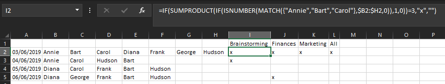
There are three types of meetings: Brainstorming, Finances and Marketing.
For Brainstorming we need Annie, Bart and Carol. For Finances we need Diana, Frank and George. For Marketing we need Annie, Diana and Hudson.
Say we have a sheet in which a range of cells represents "Monday 3rd", another represents "Tuesday 4th" and so on; in those, everyone who's available on that day has their name on it.
So, on another sheet, we'd have a formula that'd check who's available on the "Monday 3rd" by checking whose names are there. If Annie, Bart and Carol are available, we could have a Brainstorming meeting. If, otherwise, Diana, Frank and George are available, it could be a Finances one. If all six of them are available, could be either one.
Does anyone have any idea on how to do this on Excel?
So, I have a little experience in programming and (very) little experience with Excel.
What I want to do is to have a multiple condition check in a single cell, so it returns one string if a range of cells contains specific other strings, another string if it contains another set of specific strings, and so forth.
An example to make it clearer:
Let's say the purpose of this is to schedule different types of meetings according to people's availability.
There are three types of meetings: Brainstorming, Finances and Marketing.
For Brainstorming we need Annie, Bart and Carol. For Finances we need Diana, Frank and George. For Marketing we need Annie, Diana and Hudson.
Say we have a sheet in which a range of cells represents "Monday 3rd", another represents "Tuesday 4th" and so on; in those, everyone who's available on that day has their name on it.
So, on another sheet, we'd have a formula that'd check who's available on the "Monday 3rd" by checking whose names are there. If Annie, Bart and Carol are available, we could have a Brainstorming meeting. If, otherwise, Diana, Frank and George are available, it could be a Finances one. If all six of them are available, could be either one.
Does anyone have any idea on how to do this on Excel?
") glad you figured it out. Take care!
glad you figured it out. Take care!


