Help with formula please.

[MrsFrankieH]

Hello everyone,
My computer is Dell and my operating system is Windows 10.
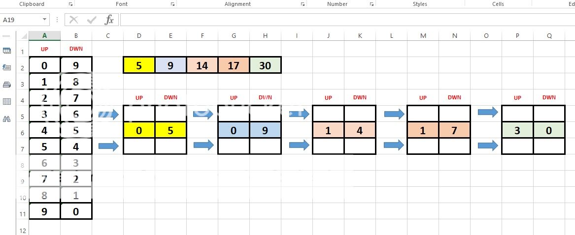
My goal is to be able to paste numbers in cells (in this example cells D2 to H2) and have appropriate numbers populate the target cells (cells above and below colored cells). I don't know the appropriate terminology to explain so this is what the cells look like after I've used a rudimentary formula. The formula I used to populate the middle (colored) cells are D6=INT(D2/10), E6=MOD (D2,10), G6=INT(E2/10), H6=MOD(E2,10), ...etc.

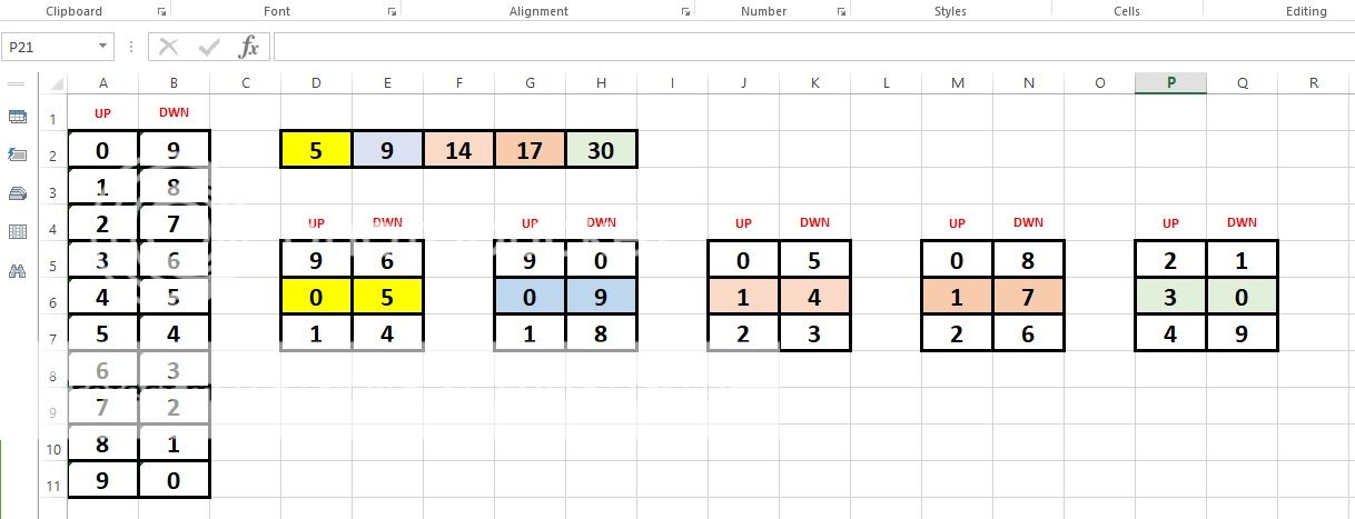
On the left are the numbers used to populate the cells above and below. For example, in the first box in yellow, the number in the first yellow cell is "0", so the number above "0" would be "9" and the number below "0" would be "1". In the next yellow box over, the number is "5", so looking at the chart on the side, the number above "5" would be "6" and the number below "5" would be "4". The same process would be repeated in the the other colored cells.​

I hope I was able to explain what I need help with. I don't have the terminology to explain it like I'd like to.
Thank you so much in advance.

 

[sheetspread]

If you don't feel like typing or pasting the formulas you can run this code on a copy of your sheet:

Sub formulapaste()
Range("D5").Value = "=INDEX($A$2:$A$11,IFERROR(1/(1/(MATCH(D6,$A$2:$A$11,0)-1)),10))"
Range("E5").Value = "=INDEX($B$2:$B$11,IFERROR(1/(1/(MATCH(E6,$B$2:$B$11,0)-1)),10))"
Range("D6").Value = "=INT(D2/10)"
Range("E6").Value = "=MOD(D2,10)"
Range("D7").Value = "=INDEX($A$2:$A$11,MOD(MATCH(D6,$A$2:$A$11,0),10)+1)"
Range("E7").Value = "=INDEX($B$2:$B$11,MOD(MATCH(E6,$B$2:$B$11,0),10)+1)"
Range("G5").Value = "=INDEX($A$2:$A$11,IFERROR(1/(1/(MATCH(G6,$A$2:$A$11,0)-1)),10))"
Range("H5").Value = "=INDEX($B$2:$B$11,IFERROR(1/(1/(MATCH(H6,$B$2:$B$11,0)-1)),10))"
Range("G6").Value = "=INT(E2/10)"
Range("H6").Value = "=MOD(E2,10)"
Range("G7").Value = "=INDEX($A$2:$A$11,MOD(MATCH(G6,$A$2:$A$11,0),10)+1)"
Range("H7").Value = "=INDEX($B$2:$B$11,MOD(MATCH(H6,$B$2:$B$11,0),10)+1)"
Range("J5").Value = "=INDEX($A$2:$A$11,IFERROR(1/(1/(MATCH(J6,$A$2:$A$11,0)-1)),10))"
Range("K5").Value = "=INDEX($B$2:$B$11,IFERROR(1/(1/(MATCH(K6,$B$2:$B$11,0)-1)),10))"
Range("J6").Value = "=INT(F2/10)"
Range("K6").Value = "=MOD(F2,10)"
Range("J7").Value = "=INDEX($A$2:$A$11,MOD(MATCH(J6,$A$2:$A$11,0),10)+1)"
Range("K7").Value = "=INDEX($B$2:$B$11,MOD(MATCH(K6,$B$2:$B$11,0),10)+1)"
Range("M5").Value = "=INDEX($A$2:$A$11,IFERROR(1/(1/(MATCH(M6,$A$2:$A$11,0)-1)),10))"
Range("N5").Value = "=INDEX($B$2:$B$11,IFERROR(1/(1/(MATCH(N6,$B$2:$B$11,0)-1)),10))"
Range("M6").Value = "=INT(G2/10)"
Range("N6").Value = "=MOD(G2,10)"
Range("M7").Value = "=INDEX($A$2:$A$11,MOD(MATCH(M6,$A$2:$A$11,0),10)+1)"
Range("N7").Value = "=INDEX($B$2:$B$11,MOD(MATCH(N6,$B$2:$B$11,0),10)+1)"
Range("P5").Value = "=INDEX($A$2:$A$11,IFERROR(1/(1/(MATCH(P6,$A$2:$A$11,0)-1)),10))"
Range("Q5").Value = "=INDEX($B$2:$B$11,IFERROR(1/(1/(MATCH(Q6,$B$2:$B$11,0)-1)),10))"
Range("P6").Value = "=INT(H2/10)"
Range("Q6").Value = "=MOD(H2,10)"
Range("P7").Value = "=INDEX($A$2:$A$11,MOD(MATCH(P6,$A$2:$A$11,0),10)+1)"
Range("Q7").Value = "=INDEX($B$2:$B$11,MOD(MATCH(Q6,$B$2:$B$11,0),10)+1)"
End Sub

 

[MrsFrankieH]

Hi Spreadsheet!! I'm going to run a repair on my Excel and try again, i think that's the problem.

 

[MrsFrankieH]

That looks impressive Spreadsheet!! I've never done codes before. I'm going to have to look up where to put it. Thank you so much!! It's another weapon in my arsenal.

 

[sheetspread]

Maybe my Excel is corrupted?

Be sure everything matches exactly. There are spaces between your cells so simply dragging over will distort many of the references.

 

[sheetspread]

I've never done codes before.

Type alt-f11, paste the code, and run (via the play button or F5 key)

 

[Eric W]

Looks like I was a bit hasty when I posted my original formulas. The second formulas for each color should have been reversed:

Excel 2012

	A	B	C	D	E	F	G	H	I	J	K
1	Up	Down
2	0	9		5	9	14	17	30
3	1	8
4	2	7		Up	Down		Up	Down		Up	Down
5	3	6		9	6		9	0		0	5
6	4	5		0	5		0	9		1	4
7	5	4		1	4		1	8		2	3
8	6	3
9	7	2
10	8	1
11	9	0

<tbody>
</tbody>

Sheet9
​

Worksheet Formulas Cell Formula D5 =MOD(D6-1,10) E5 =MOD(E6+1,10) G5 =MOD(G6-1,10) H5 =MOD(H6+1,10) J5 =MOD(J6-1,10) K5 =MOD(K6+1,10) D7 =MOD(D6+1,10) E7 =MOD(E6-1,10) G7 =MOD(G6+1,10) H7 =MOD(H6-1,10) J7 =MOD(J6+1,10) K7 =MOD(K6-1,10) <tbody> </tbody>

<tbody>
</tbody>

And as far as using the lookup tables, the way I interpret your request is that you want the values surrounding the value in row 6 in the specified table. If so, try this:

Excel 2012

	A	B	C	D	E	F	G	H	I	J	K	L	M	N	O	P	Q
1	Up	Down
2	0	9		5	9	14	17	30
3	1	8
4	2	7		Up	Down		Up	Down		Up	Down		Up	Down		Up	Down
5	3	6		9	6		9	0		0	5		0	8		2	1
6	4	5		0	5		0	9		1	4		1	7		3	0
7	5	4		1	4		1	8		2	3		2	6		4	9
8	6	3
9	7	2
10	8	1
11	9	0

<tbody>
</tbody>

Sheet9
​

Worksheet Formulas Cell Formula D5 =INDEX($A$2:$B$11,MOD(MATCH(D6,INDEX($A$2:$B$11,0,MATCH(D$4,$A$1:$B$1,0)),0)-2,10)+1,MATCH(D$4,$A$1:$B$1,0)) D7 =INDEX($A$2:$B$11,MOD(MATCH(D6,INDEX($A$2:$B$11,0,MATCH(D$4,$A$1:$B$1,0)),0),10)+1,MATCH(D$4,$A$1:$B$1,0)) <tbody> </tbody>

<tbody>
</tbody>

Copy the D5 formula to all the row 5 cells, and copy the D7 formula to all the row 7 cells. (I tested them all this time!)

 

[MrsFrankieH]

Type alt-f11, paste the code, and run (via the play button or F5 key)

Thank you Spreadsheet, I checked to make sure everything is lined up and I'm practicing with the codes. This is how i learn. Thanks again for everything!!!

 

[MrsFrankieH]

Looks like I was a bit hasty when I posted my original formulas. The second formulas for each color should have been reversed:

Excel 2012

	A	B	C	D	E	F	G	H	I	J	K
1	Up	Down
2	0	9		5	9	14	17	30
3	1	8
4	2	7		Up	Down		Up	Down		Up	Down
5	3	6		9	6		9	0		0	5
6	4	5		0	5		0	9		1	4
7	5	4		1	4		1	8		2	3
8	6	3
9	7	2
10	8	1
11	9	0

<tbody>
</tbody>

Sheet9
​

Worksheet Formulas Cell Formula D5 =MOD(D6-1,10) E5 =MOD(E6+1,10) G5 =MOD(G6-1,10) H5 =MOD(H6+1,10) J5 =MOD(J6-1,10) K5 =MOD(K6+1,10) D7 =MOD(D6+1,10) E7 =MOD(E6-1,10) G7 =MOD(G6+1,10) H7 =MOD(H6-1,10) J7 =MOD(J6+1,10) K7 =MOD(K6-1,10) <tbody> </tbody>

<tbody>
</tbody>

And as far as using the lookup tables, the way I interpret your request is that you want the values surrounding the value in row 6 in the specified table. If so, try this:

Excel 2012

	A	B	C	D	E	F	G	H	I	J	K	L	M	N	O	P	Q
1	Up	Down
2	0	9		5	9	14	17	30
3	1	8
4	2	7		Up	Down		Up	Down		Up	Down		Up	Down		Up	Down
5	3	6		9	6		9	0		0	5		0	8		2	1
6	4	5		0	5		0	9		1	4		1	7		3	0
7	5	4		1	4		1	8		2	3		2	6		4	9
8	6	3
9	7	2
10	8	1
11	9	0

<tbody>
</tbody>

Sheet9
​

Worksheet Formulas Cell Formula D5 =INDEX($A$2:$B$11,MOD(MATCH(D6,INDEX($A$2:$B$11,0,MATCH(D$4,$A$1:$B$1,0)),0)-2,10)+1,MATCH(D$4,$A$1:$B$1,0)) D7 =INDEX($A$2:$B$11,MOD(MATCH(D6,INDEX($A$2:$B$11,0,MATCH(D$4,$A$1:$B$1,0)),0),10)+1,MATCH(D$4,$A$1:$B$1,0)) <tbody> </tbody>

<tbody>
</tbody>

Copy the D5 formula to all the row 5 cells, and copy the D7 formula to all the row 7 cells. (I tested them all this time!)

Thank you Eric!!! I really your help and hard work! I appreciate it very much!! Thanks again!