Data validation - dynamic and also dependent on a particular column

realdemigod

Board Regular
Joined
Aug 19, 2014
Messages
51
Office Version
  1. 365
Platform
  1. MacOS
Hi,
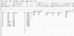
Please refer to the image in the link below. I’m trying to create a data validation that lets a user choose Product and Colour of a car from the Manufacturer.


Is there way to put some function in data validation list option so that it looks for Audi on the worksheet and takes the Product as the first list and then second data validation show the list of colours again the product types (Q7 and Q5)


For example data validation at A1 should show Q7 and Q5 and then at B1 should show the corresponding colours against each model for Audi. The range could be anywhere in the particular columns but the placements of the columns are fixed. So defining a name would be a challenge.

I can't use any macro. Is it possible with some if or some other function?

HTML:
https://imgur.com/aevnBpg

Thanks
 
I'm still not 100% sure I know what you're trying to do so I won't try and give you a solution but I will give hints.

Earlier you said you were trying to construct the formula
=COUNTIF($C3:$C$20,C3)
where you didn't know the row but you could use MATCH and gave the example: "=ADDRESS(MATCH("Audi",C1:C20,0),CELL("col",C1))"

Hint: The ADDRESS function has another parameter option, so try option 3:
=ADDRESS(MATCH("Audi",C1:C20,0),COLUMN(C1),3)

I'm guessing you may start using INDIRECT but if you need to also find the number of rows where the manufacturer is specified then constructing it may need COUNTA, SEARCH and MID.

Good luck!
 
Upvote 0

Excel Facts

Will the fill handle fill 1, 2, 3?
Yes! Type 1 in a cell. Hold down Ctrl while you drag the fill handle.
I'm still not 100% sure I know what you're trying to do so I won't try and give you a solution but I will give hints.

Earlier you said you were trying to construct the formula
=COUNTIF($C3:$C$20,C3)
where you didn't know the row but you could use MATCH and gave the example: "=ADDRESS(MATCH("Audi",C1:C20,0),CELL("col",C1))"

Hint: The ADDRESS function has another parameter option, so try option 3:
=ADDRESS(MATCH("Audi",C1:C20,0),COLUMN(C1),3)

I'm guessing you may start using INDIRECT but if you need to also find the number of rows where the manufacturer is specified then constructing it may need COUNTA, SEARCH and MID.

Good luck!

Hello Toadstool,
Thanks. Your solution is perfect it is working fine but the major thing before I can implement is to know on which row Audi starts in the worksheet I have. In the sample file it starts at row 3 but in the working file I have is 1000s of rows and I need to find out where Audi begins first. Once I know then I can use it in the first argument in the COUNTIF function for the column E you gave.

One thing I know for sure is Audi always exists in one particular column, it never changes as it is an output file from an ERP system. Let's say Audi and other manufacturers are always in column AB but I don't know where it starts every time the worksheet gets updated. With MATCH function I can find out the row, so let's say it starts at 133, so AB133 is the first instance of Audi in the column AB in the worksheet. Now I can replace $C3 with $AB133 in the COUNTIF function.

There is no way I know through which I can use my knowledge that column is always AB along with the returned value for the first instance from MATCH function together to make it $AB (row number)<rowno.>. I'm struggling to achieve that as your solution needs to know beforehand if Audi will start at C3 or C4 or any other row in the column C.</rowno.>
 
Last edited:
Upvote 0
Here is the file. You can ignore the columns after the third one (manufacturer). Thanks


I'm not clear what you want.
Do you want 3 cells with DV (Data Validation), for Manufacturer, Product and Color where you can select what you want?
And will the DV cells be in the cascade?
Or do you want 2 cells with DV (Data Validation), cascaded, for Manufacturer and Product and in the COLOR column to list all the colors related to the selections from Manufacturer and Product?
Are these columns of interest (A, B, and C)? who have data on Manufacturer, Prouct and Color?
 
Upvote 0
I'm sorry but I can't follow what you're saying.

Sorry for the confusion. Now I know why you got confused as the AGGREGATE function does not need the object in question to be at a particular row. I was doing some research on it and found a good video. Now I know how to get what I'm looking for.
 
Upvote 0
You're welcome!

Let me give the 5 cent tour...

I don't want to base my Manufacturer LoV on all of column C otherwise you'd offer a list of 6 Audi then 6 BMW.
To limit this my E3 formula says "Count how many of cell C3 are in cells C3 to C20" and of course the answer is 6, but the formula doesn't lock the starting row so when I copy down then in E4 it only looks in E4 to E20, so returns 5. This means the last entry for a Manufacturer will always have a count of 1 (cells E8 and E14).

Now my H3 formula says INDEX into the manufacturer with a row of the AGGREGATE which checks for any E$3:E$20=1.
The AGGREGATE is using the 15 option of SMALL so I can select the 1st, then the 2nd, 3rd, etc. match to that 1 value by specifying which I want. I do this with the H3 formula using ROWS(H$2:H2) part so ROWS says 1 for the first occurrence but as it's copied down that changes to ROWS(H$2:H3) which returns a 2 so I get the 2nd value of 1 which is in the BMW row.

Column F is concatenating Model and Manufacturer so I can avoid issues with Mazda Yaris and Toyota Yaris.

Column G is similar to column E but I'm counting down the Product only when the Manufacturer matches the one selected in K3 LoV.

The I3 and down formula is the same as H3 but looking for a 1 down column G.

The N3 and down is another INDEX and SMALL option of AGGREGATE but checking column F for rows where the concatenated Product and Manufacturer match those already selected from my K3 and L3 dynamic LoVs.


OK, well that was more like a 10 cents tour but I hope it helps.

Hello Toadstool,
Apologies in advance for not following up sooner (Swiss bosses travel a lot). Your solution is working fine but I confused you so much didn't want to bother you anymore so I tried to do manually some changes that are exactly needed for my work. Please refer to the file on box. To avoid more confusion I'm sharing the file you shared with me with your solution.

In the col. I the product listing for Audi is fine but X3 and X5 for BMW are not showing up. As I need to replicate K3, M3 and L3, for BMW as well I tried different things but in the data validations I created on K4, L4 and M4, I still see product listing related to Audi and the colours related to Audi.

I tried to tweak the col. N but to no avail.

Really appreciate if you could help me again!
 

Attachments

  • dependent list.png
    dependent list.png
    79.6 KB · Views: 8
Upvote 0
Realdemigod,

I understand the elapsed time. Too much Toblerone can make you lose track... ;)

The dropbox had multiple LoV's for selection which my original design won't handle and there were a couple of cells where the formulae had been deleted.

I have restructured the sheet to better describe its use.
"---Selections---" is where you select the LoV for the specification. Only one row of selections is supported.
"---Data---" is where you can add your Product, Colour and Manufacturer
"---Worker Columns---" is a work area where you should not make any changes.

If you need changes (e.g. allow multiple LoV selections) let me know and I'll redesign the sheet to support.

Book1
ABCDEFGHIJKLMN
1--- Selections ------ Data ------ Worker Columns ---
2ProductColourManufacturer$L$4:$L$5$M$4:$M$5$N$4:$N$6
3ManufacturerProductSelect ColourQ7WhiteAudiManUManProdProdUManProdColors
4BMWX3MagentaQ7BlueAudi6Q7Audi AudiX3Grey
5Q7RedAudi5Q7Audi BMWX5Magenta
6Q7BlackAudi4Q7Audi   Florescent
7Q5BlueAudi3Q7Audi    
8Q5WhiteAudi2Q5Audi    
9X3GreyBMW1Q5Audi    
10X3MagentaBMW6X3BMW3   
11X3FlorescentBMW5X3BMW2   
12X5TealBMW4X3BMW1   
13X5BabyBlueBMW3X5BMW3   
14X5StarkWhiteBMW2X5BMW2   
151X5BMW1   
Master
Cell Formulas
RangeFormula
L2:N2L2=ADDRESS(ROW(L4),COLUMN())&":"&ADDRESS(ROW(L4)+COUNTIF(L4:L44,"> ")-1,COLUMN())
I4:I15I4=COUNTIF($G3:$G$20,G3)
J4:J15J4=E3&G3
K4:K15K4=IF(G3=A$4,COUNTIF($J4:$J$21,E3&G3),"")
L4:L15L4=IF(COUNTIF(I:I,1)<ROWS(L$3:L3),"",INDEX(G$3:G$20,AGGREGATE(15,6,ROW(I$4:I$21)-ROW(L$3)/(I$4:I$21=1),ROWS(L$3:L3))))
M4:M15M4=IF(COUNTIF(K:K,1)<ROWS(M$3:M3),"",INDEX(E$3:E$20,AGGREGATE(15,6,ROW(J$4:J$21)-ROW(M$3)/(K$4:K$21=1),ROWS(M$3:M3))))
N4:N15N4=IF(COUNTIF($J$4:$J$21,B$4&A$4)<ROWS(N$3:N3),"",INDEX(F$3:F$20,AGGREGATE(15,6,ROW(N$4:N$21)-ROW(N$3)/(J$4:J$21=B$4&A$4),ROWS(N$3:N3))))
Cells with Data Validation
CellAllowCriteria
A4List=INDIRECT($L$2)
B4List=INDIRECT($M$2)
C4List=INDIRECT($N$2)
 
Upvote 0
Realdemigod,

I understand the elapsed time. Too much Toblerone can make you lose track... ;)

The dropbox had multiple LoV's for selection which my original design won't handle and there were a couple of cells where the formulae had been deleted.

I have restructured the sheet to better describe its use.
"---Selections---" is where you select the LoV for the specification. Only one row of selections is supported.
"---Data---" is where you can add your Product, Colour and Manufacturer
"---Worker Columns---" is a work area where you should not make any changes.

If you need changes (e.g. allow multiple LoV selections) let me know and I'll redesign the sheet to support.

Thanks a lot Toadstool, appreciate your quick help! :)

The data validations on A4,B4 and C4 are fine but if I replicate the same data validations with the criteria you gave, on the next row, I am still struggling to populate as needed. For example

Row 4 - Audi ->Q7->Blue
Row 5 -> BMW -> instead of X3, X5 as drop downs, I still see Q5, Q7 from the row above. But once I change the row 4 to BMW on A4, I can see X3 and X5 on B5.
 
Upvote 0
Realdemigod,

Ah! That won't work. My solution will only support one entry because it builds the Data Validation List based on the previous selection (i.e. if you select BMW then column M for the Product will only show BMW Products).

I can't see how to do this using just functions when you want multiple rows of the three LoVs. I suspect you may need to resort to VBA.

Sorry!

It is ok, thanks for your help. But I'm seeing some videos on YouTube on dependent validations and I don't know if combinations of functions like OFFSET, INDEX and AGGREGATE can be used to populate the data validations. I'm sure many people who work with excel would have come across this issue at some point.
 
Upvote 0

Forum statistics

Threads
1,214,385
Messages
6,119,209
Members
448,874
Latest member
b1step2far

We've detected that you are using an adblocker.

We have a great community of people providing Excel help here, but the hosting costs are enormous. You can help keep this site running by allowing ads on MrExcel.com.
Allow Ads at MrExcel

Which adblocker are you using?

Disable AdBlock

Follow these easy steps to disable AdBlock

1)Click on the icon in the browser’s toolbar.
2)Click on the icon in the browser’s toolbar.
2)Click on the "Pause on this site" option.
Go back

Disable AdBlock Plus

Follow these easy steps to disable AdBlock Plus

1)Click on the icon in the browser’s toolbar.
2)Click on the toggle to disable it for "mrexcel.com".
Go back

Disable uBlock Origin

Follow these easy steps to disable uBlock Origin

1)Click on the icon in the browser’s toolbar.
2)Click on the "Power" button.
3)Click on the "Refresh" button.
Go back

Disable uBlock

Follow these easy steps to disable uBlock

1)Click on the icon in the browser’s toolbar.
2)Click on the "Power" button.
3)Click on the "Refresh" button.
Go back
Back
Top