Dynamically Pulling Data between Worksheets

[AGMGCM]

Hello,

I am trying to do a small pull of data between two worksheets but in an active manner, I'm hoping someone here might be able to figure this one out as I can't come up with a perfect solution.

Sample Data on Worksheet1:

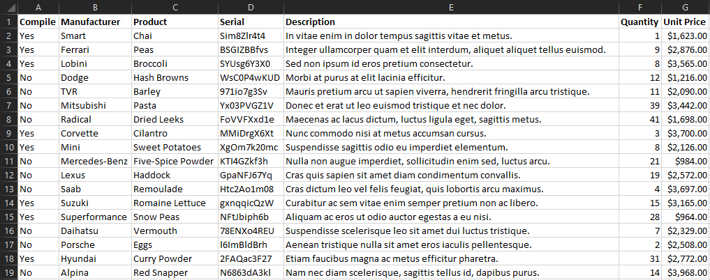
On Worksheet2 I would like to pull anything that says 'Yes' in Worksheet1's Column A - this is using a data validation list of Yes/No

Desired results for Worksheet2:

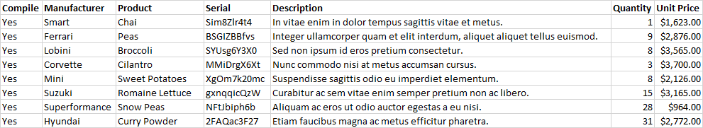
I would like this to be dynamic so that anything switched to Yes shows up on Worksheet2 and when it switches to No, it disappears from Worksheet2. I understand that something like this could be done in Access but I would like to keep this in Excel if possible.

Thank you

 

[Toadstool]

Hello,

If this is Worksheet1

	A	B	C	D
1	Compile	Manufacturer	Product	Price
2	Yes	White Sky Inc.	Solar flashlight	$ 22.83
3	No	Easy Partners	Rubber ladder	$ 12.32
4	No	ACME Widgets	Cat trainer	$ 9.00
5	Yes	Hope & Sky Inc.	Tissue umbrella	$ 230.22

<tbody>
</tbody>

Worksheet1​

Then this formulae should work:
=IF(COUNTIF(Worksheet1!$A$2:$A$20,"Yes") < ROWS(A$1:A1),"",INDEX(Worksheet1!A$2:A$20,AGGREGATE(15,6,ROW(Worksheet1!$A$2:$A$20)-ROW(Worksheet1!$A$1)/(Worksheet1!$A$2:$A$20="Yes"),ROWS(A$1:A1))))

Put it in Worksheet2 cell A2. Change the $20 to the maximum row number you'll ever have (say $9999) and copy it down that many rows. Now highlight those cells and copy across the number of columns where you have data.

	A	B	C	D
1	Compile	Manufacturer	Product	Price
2	Yes	White Sky Inc.	Solar flashlight	22.83
3	Yes	Hope & Sky Inc.	Tissue umbrella	230.22
4

<tbody>
</tbody>

Worksheet2​

Worksheet Formulas Cell Formula A2 =IF(COUNTIF(Worksheet1!$A$2:$A$20,"Yes") < ROWS(A$1:A1),"",INDEX(Worksheet1!A$2:A$20,AGGREGATE(15,6,ROW(Worksheet1!$A$2:$A$20)-ROW(Worksheet1!$A$1)/(Worksheet1!$A$2:$A$20="Yes"),ROWS(A$1:A1)))) B2 =IF(COUNTIF(Worksheet1!$A$2:$A$20,"Yes") < ROWS(B$1:B1),"",INDEX(Worksheet1!B$2:B$20,AGGREGATE(15,6,ROW(Worksheet1!$A$2:$A$20)-ROW(Worksheet1!$A$1)/(Worksheet1!$A$2:$A$20="Yes"),ROWS(B$1:B1)))) <tbody> </tbody>

<tbody>
</tbody>

 

[My Aswer Is This]

The first part of your request would be simple:
But the second part about deleting the row from Sheet(2) would be more complicated.
Will the value on Sheet(2) column A change to "No" or did you mean if the value in column A of sheet(1) changes to "No"

If it's when value on sheet(1) changes to "No" how would we know what row on sheet(2) to Delete.
Is their any unique value on the row to identify the row.
If you mean when "No" in entered into column A of Sheet(2) it would be simple.


Here is the way to do the first part:

This is an auto sheet event script
Your Workbook must be Macro enabled
To install this code:
Right-click on the sheet (1) Tab
Select View Code from the pop-up context menu
Paste the code in the VBA edit window

When you enter "Yes" into column A of Sheet(1) the script will run.

Private Sub Worksheet_Change(ByVal Target As Range)
'Modified  8/25/2019  12:49:26 AM  EDT
If Target.Column = 1 And Target.Value <> "" Then
If Target.Cells.CountLarge > 1 Or IsEmpty(Target) Then Exit Sub
Dim lastrow As Long
lastrow = Sheets(2).Cells(Rows.Count, "A").End(xlUp).Row + 1
    Select Case Target.Value
        Case "Yes"
        Rows(Target.Row).Copy Sheets(2).Rows(lastrow)
        Case "No"
    
    End Select
End If
End Sub

 

[Peter_SSs]

I would take a somewhat similar approach to Toadstool but there are quite a lot of things being calculated multiple time in that suggestion so I have used a helper column & helper cell to save calculating so much.

Here is my Worksheet1 with just some random numbers as dummy data in columns B:G (We cannot copy your sample data from images like you posted. See my signature block below for help on how to post data that can be copied - like Toadstool & I have done in this thread)

Column H is my helper column but it could be any column & it could be hidden after entering the formulas.
Cell H1 is left empty
Formula in H2 is copied down to the end of your data or the end of wherever your data might eventually come to.

Excel Workbook
	A	B	C	D	E	F	G	H
2	No	83	24	71	45	68	80	0
3	No	50	21	1	29	95	51	0
4	Yes	89	33	11	95	3	53	1
5	Yes	56	76	89	98	96	50	2
6	No	11	52	24	31	89	97	2
7	Yes	93	53	25	12	31	59	3
8	No	33	40	65	51	97	50	3
9	Yes	5	63	50	87	43	43	4
10	No	30	19	84	83	30	98	4
11	Yes	57	2	78	79	68	43	5
12	No	76	74	7	36	15	8	5
13	No	13	3	7	47	99	20	5
14	Yes	10	95	87	64	5	30	6
15	No	88	14	28	26	2	58	6
16	Yes	4	18	90	6	93	40	7
17	No	65	3	62	56	42	55	7
18	No	90	20	12	12	86	14	7
19	No	8	1	54	64	30	27	7
20								7
21								7
Worksheet1

In Worksheet2 I have used cell Z1 as a helper cell. Again it could be another cell & the column can be hidden if you want.
Formula in A2 is copied down as far as you might ever need.
Formula in B2 is copied (after adjusting the max row $1000 if needed) across and down as far as column A was.

Excel Workbook
	A	B	C	D	E	F	G	H	I	Z
1										7
2	Yes	89	33	11	95	3	53
3	Yes	56	76	89	98	96	50
4	Yes	93	53	25	12	31	59
5	Yes	5	63	50	87	43	43
6	Yes	57	2	78	79	68	43
7	Yes	10	95	87	64	5	30
8	Yes	4	18	90	6	93	40
9
10
Worksheet2