Coontradis
New Member
- Joined
- Aug 28, 2019
- Messages
- 1
For the pros…
Been working on this for the last day….
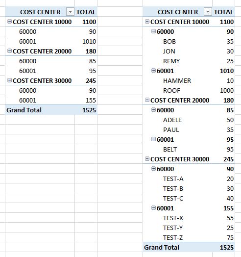
I have a monthly report that update each week. It consists of cost center and account number. I want to control the budget and have the total of each account for each cost center. Not very complicated up to now… Here is the fun part: I have 5 cost center. In each cost center I have accounts. The accounts numbers are the same for all cost center. Ex: account 60000 is for my labor, so I have a 60000 account in my production cost center, service, office, sales and maintenance.
I want to have a tab for each of my cost center that give me the total of the account. But here is how the data are coming from the download.:
<tbody>
</tbody>
SO for account 60000 (column C) for cost center 10000 (column B) I want the total as show in row 4 column I (total by account for a specific cost center).
The data of the cost center are always in column B but appear only once where the data for this cost center start. The account stands in column C and the total in I.
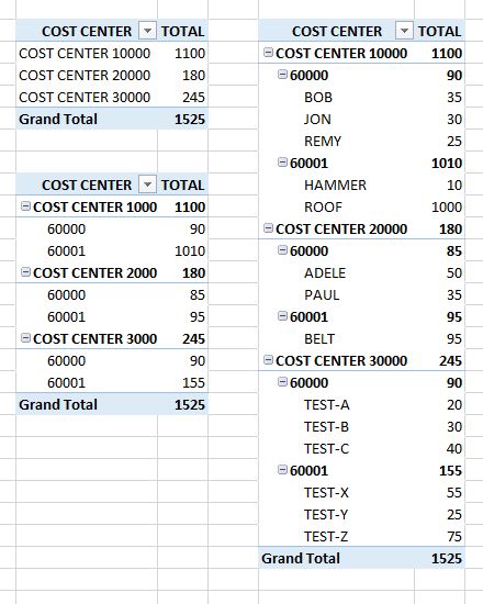
I would like to have the total of each account in another tab (on for each cost center). Note that the data add every week so this need to be dynamic. I also work with excel 2016
Thanks for helping me
Been working on this for the last day….
I have a monthly report that update each week. It consists of cost center and account number. I want to control the budget and have the total of each account for each cost center. Not very complicated up to now… Here is the fun part: I have 5 cost center. In each cost center I have accounts. The accounts numbers are the same for all cost center. Ex: account 60000 is for my labor, so I have a 60000 account in my production cost center, service, office, sales and maintenance.
I want to have a tab for each of my cost center that give me the total of the account. But here is how the data are coming from the download.:
| A | B | C | D | E | F | G | H | I | |
| 1 | COST CENTER 10000 | 60000 | REMY | 25 | |||||
| 2 | JON | 30 | |||||||
| 3 | BOB | 30 | |||||||
| 4 | Result | 85 | |||||||
| 5 | 60001 | Hammer | 10 | ||||||
| 6 | Roof | 1000 | |||||||
| 7 | Result | 1010 | |||||||
| 8 | Result | 1095 | |||||||
| 9 | Cost center 20000 | 60000 | Paul | 35 | |||||
| 10 | Adele | 50 | |||||||
| 11 | Result | 85 | |||||||
| 12 | 60001 | Belt | 95 | ||||||
| 13 | |||||||||
| 14 |
<tbody>
</tbody>
SO for account 60000 (column C) for cost center 10000 (column B) I want the total as show in row 4 column I (total by account for a specific cost center).
The data of the cost center are always in column B but appear only once where the data for this cost center start. The account stands in column C and the total in I.
I would like to have the total of each account in another tab (on for each cost center). Note that the data add every week so this need to be dynamic. I also work with excel 2016
Thanks for helping me
")