First time creating macros for complicated sorting

AyEmmKay

New Member
Joined
Sep 26, 2019
Messages
6
Hey, all! Just a bit of background:

I work in sales at a hotel. I've been tasked with manually entering our numbers into a new system until it interfaces with the program the front desk uses to keep track of rooms. It's daunting. I'm given an extremely dense Excel file with information about the groups that stay at the hotel, the dates they stay, and the number of rooms they use per night. I'm trying to figure out how to do a combination of between and within group sorting. I feel like a visual, extremely simplified, example is best:

https://imgur.com/rNNQu1o

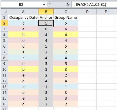
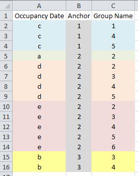
The first set is the original data, completely randomized just for example's sake. The second set is sorted E then D, so it'd be like Occupancy Date then Group Name. This results in the Occupancy Date being in order, but the Group Names are not grouped. The third set is sorted G then H, so it'd be like Group Name then Occupancy Date. This results in the Group Names being grouped together, but it's not in chronological order. The fourth set is how I'd like it to come out. The Group Names are grouped together, they progress from one grouping to the next based on initial Occupancy Date, and they progress within the groupings in chronological order.

I don't even know where to start, to be completely honest. I've never had to create macros before, though I get the gist. I could easily do simple things to rid the sheet of extra data that I don't need. I have no idea how to touch the grouping/sorting, though.

I'm still trying small things to get it to work like I'd want, but I figured macros would be the way to go.

Although I'm definitely asking for help, I also want to learn and understand. I get the feeling Excel is going to be my bff for a while so I want to learn how to use it properly.

Thanks a billion times over!


Excel Facts

Copy formula down without changing references
If you have =SUM(F2:F49) in F50; type Alt+' in F51 to copy =SUM(F2:F49) to F51, leaving the formula in edit mode. Change SUM to COUNT.
Hi there, here's one method... I've entered an extra column into your data, called Anchor (for want of a better name), it's in grey in column B below:

LK0C2hE.jpg


The formula in column B is =IF(A2<>A1,C2,B1)
The formula is dragged down through all rows. It's comparing the row's Occupancy Date with that of the row above, and if it's different then it grabs the Group Name from its own row; otherwise it copies the Anchor data from the row above. The result doesn't mean anything, until the sorting starts...

The following macro uses three simple sort commands, one after the other. We sort using column C, then A, then B:

Sub sorter()
Columns("A:C").Sort key1:=Range("C1"), order1:=xlAscending, Header:=xlYes
Columns("A:C").Sort key1:=Range("A1"), order1:=xlAscending, Header:=xlYes
Columns("A:C").Sort key1:=Range("B1"), order1:=xlAscending, Header:=xlYes
End Sub


The result is as desired:

1oyJtgL.jpg
 
Upvote 0
That makes a LOT of sense. I'm super new to this so I had no idea how to even approach it logically. An anchor column never occurred to me.

I'm going to give this a shot with my data as the example was extremely simplified. Not that I doubt you, but I'll let you know when/if it works.

Sincerely, thank you. You've likely made my job SO MUCH faster and easier. I'd give you a cookie if I could! :)
 
Upvote 0
Ace, glad I could help. Let me know if you run into problems and we can try work it out together. Instead of using Columns("A:C"), you could absolutely use an explicit range, such as Range("A1:Z1000")... or you could have the code figure out the range dynamically, based on your own rules.

Also you could potenially achieve the 'anchor' solution via code instead of the extra column. But it could require significant extra code. In fact, if you did need to do that, it'd probably be easiest to have the code automatically generate the anchor column; use it; then delete it again.

What I love about having multiple sorting steps is the fact you have to run the steps in reverse to get to your destination. I love the logic - it feels weird and then magic when you get the result.
 
Last edited:
Upvote 0
The word "magic" definitely crossed my mind. I had to finish up some tasks at work and fly out to take care of some stuff, so I didn't get the chance to try it out. It'll be one of the first things I do tomorrow morning, though!

If you're willing, could you walk me through your thought process step by step? I think I get it, but I'm just not used to the language. I haven't used logic like that since high school. Shame, shame, I know.
 
Upvote 0
Oh, crud. I just noticed something and I'm so sorry. I guess I'm just missing things because I've been thinking about it and twisting my mind in knots about it. I also need the Occupancy Date to end up in chronological order as well. I guess in the case of the example you used up there, it would be alphabetical. So I guess it's that I need column A in order descending, and then the values in column C descending within the groupings created by column A? Again, I'm sorry. I just don't know the language to use to communicate it.
 
Upvote 0
OH WAIT NO YOU'RE AN ANGEL! It's perfect! I was getting confused because I was looking at the group names as the letters and the dates as the numbers. You switched them and that messed me all up because I'm silly sometimes. BUT I GET IT NOW! I am forever indebted to you!
 
Upvote 0
Welcome to the MrExcel board!

If I have understood correctly, I think you can do this with a helper column & just a single sort.
I am assuming that you do actually have dates instead of single-digit numbers & probably actual names not single letters. If so, remember that it is best not to over-simplify sample data. It is also better for you (that is more helpers & faster if you provide any sample data in a form that can be copied and pasted into a workbook to test with (like mine below). My signature block below has help with that. Unfortunately we cannot copy fro images like you (or brownbread) provided.

If my assumptions are correct then try this formula in C2, copied down then select all 3 columns and sort on the helper column. The 20 values in the formula just need to be anything bigger than the longest name likely to occur in column A.

Before sorting:


Excel 2016
ABC
1GroupDateSort
2xyz13/09/2019xyz 43721
3bbb14/09/2019bbb 43722
4kkkkk15/09/2019kkkkk 43723
5kkkkk14/09/2019kkkkk 43722
6xyz17/09/2019xyz 43725
7abcde18/09/2019abcde 43726
8kkkkk13/09/2019kkkkk 43721
9xyz14/09/2019xyz 43722
10x15/09/2019x 43723
11abcde14/09/2019abcde 43722
12kkkkk17/09/2019kkkkk 43725
13a13/09/2019a 43721
14x17/09/2019x 43725
15x14/09/2019x 43722
16abcde17/09/2019abcde 43725
Sort
Cell Formulas
RangeFormula
C2=LEFT(A2&REPT(" ",20),20)&B2


After sorting:


Excel 2016
ABC
1GroupDateSort
2a13/09/2019a 43721
3abcde14/09/2019abcde 43722
4abcde17/09/2019abcde 43725
5abcde18/09/2019abcde 43726
6bbb14/09/2019bbb 43722
7kkkkk13/09/2019kkkkk 43721
8kkkkk14/09/2019kkkkk 43722
9kkkkk15/09/2019kkkkk 43723
10kkkkk17/09/2019kkkkk 43725
11x14/09/2019x 43722
12x15/09/2019x 43723
13x17/09/2019x 43725
14xyz13/09/2019xyz 43721
15xyz14/09/2019xyz 43722
16xyz17/09/2019xyz 43725
Sort
 
Last edited:
Upvote 0

Forum statistics

Threads
1,212,929
Messages
6,110,743
Members
448,295
Latest member
Uzair Tahir Khan

We've detected that you are using an adblocker.

We have a great community of people providing Excel help here, but the hosting costs are enormous. You can help keep this site running by allowing ads on MrExcel.com.
Allow Ads at MrExcel

Which adblocker are you using?

Disable AdBlock

Follow these easy steps to disable AdBlock

1)Click on the icon in the browser’s toolbar.
2)Click on the icon in the browser’s toolbar.
2)Click on the "Pause on this site" option.
Go back

Disable AdBlock Plus

Follow these easy steps to disable AdBlock Plus

1)Click on the icon in the browser’s toolbar.
2)Click on the toggle to disable it for "mrexcel.com".
Go back

Disable uBlock Origin

Follow these easy steps to disable uBlock Origin

1)Click on the icon in the browser’s toolbar.
2)Click on the "Power" button.
3)Click on the "Refresh" button.
Go back

Disable uBlock

Follow these easy steps to disable uBlock

1)Click on the icon in the browser’s toolbar.
2)Click on the "Power" button.
3)Click on the "Refresh" button.
Go back
Back
Top