FIND Question

RudeClown

Board Regular
Joined
May 31, 2016
Messages
56
Hi! This seems like it should be pretty easy, but I can't get Excel to accept my formula. Maybe there's a better way to do what I am trying to do. There are two relevant tabs, "Total Summary" and "List." I am entering the formula on "Total Summary" to count items that meet specific criteria on "List." I want to count rows on List! where J <> the word "project" AND column Y contains the number found in Total Summary! column A. Column Y will contain a list of numbers, such as: 12, 13,14, 15, 16, 17. I am using FIND to determine if the number is present in List! Y. If not, the IFERROR should return 0, it will not be greater than zero, and it won't get counted. If it finds the number, it will return the position which will be greater than zero, and should be counted if J:J is also <> "project." The formula I am trying to use is:

=COUNTIFS(List!$J:$J,"<>Project",IFERROR(FIND($A18,List!$Y:$Y),0),">0")


Excel won't accept the formula as-is, and I'm not sure why. Any suggestions would be appreciated!
 

Excel Facts

Excel Can Read to You
Customize Quick Access Toolbar. From All Commands, add Speak Cells or Speak Cells on Enter to QAT. Select cells. Press Speak Cells.
Maybe:

=SUMPRODUCT((List!J:J<>"Project")*(List!Y:Y>0))
 
Upvote 0
Won't that count every row where there is any number > 0 in Y? What it needs to do, is only count rows where the number in Total Summary!A matches a number found in List!Y. List!Y will contain a list of numbers which may or may not contain the number I am comparing against.
 
Upvote 0
1) The FIND function looks for a specified text in a string. To search for something in a range of cells, you would need to use the MATCH function.

2) Why not just =COUNTIFS(List!$J:$J,"<>Project",List!$Y:$Y,$A18) ?
 
Upvote 0
Is one of these what you want? If not please give a small set of dummy sample data & explain in relation to that. Remember that you are very familiar with your layout, data and aim, but we are not. :)

I would try to avoid whole column references. In most cases you can select a number of rows that is plenty for the expected data but well short of the million+ rows available in Excel.

=COUNTIFS(List!$J$1:$J$2000,"<>Project",List!$Y$1:$Y$2000,A18)

=SUMPRODUCT(--(List!$J$1:$J$2000<>"Project"),--ISNUMBER(FIND(","&A18&",",","&SUBSTITUTE(List!$Y$1:$Y$2000," ","")&",")))
 
Last edited:
Upvote 0
@Tetra201 - The cells in List!Y will contain either a single number, a string which will contain several numbers (In the format: 4, 5, 6, 7, 8), or will be blank. I want the row counted if the number in Total Summary!A is found in the cell in List!Y, either by itself, or is within the list. Though, that leads me to another possible problem, will the FIND function care if it is looking for a number, versus the text equivalent? With how I am generating the output for List!Y, the single digits are numbers and the strings are text.
 
Upvote 0
@Peter_SSs: I was hoping that my explanation in my original post would provide sufficient explanation, but I apologize it did not. This particular issue is a potential partial solution within a larger problem I am trying to figure out. I would be happy to go into more detail if you guys (and/or gals) are willing to assist on the larger scale (just one somewhat complex metric I am trying to figure out, and is the last item before I can complete the project). I would be happy to provide a test file, but what is the best way to do-so here?
 
Last edited:
Upvote 0
I would be happy to provide a test file, but what is the best way to do-so here?
You cannot upload actual workbooks in this forum. In any case I am generally not a fan of working with actual workbooks from members as they often turn out to take too long to figure out what the workbook is actually about.

However, you can show small screen shots, formulas etc directly in your post as I have here. My signature block below has help on this.

From your description in post 1 and your further explanation to Tetra201 in post 6, I am not understanding in what way my second suggestion in post 5 fails to deliver what you want. Here it is in screen shot form where the formula result of 3 is counting the yellow rows from the 'List' sheet. Can you clarify what the result should be (& how you get that result) for this sample data if it is not 3?


Excel 2016
AB
1883
Total Summary
Cell Formulas
RangeFormula
B18=SUMPRODUCT(--(List!$J$1:$J$2000<>"Project"),--ISNUMBER(FIND(","&A18&",",","&SUBSTITUTE(List!$Y$1:$Y$2000," ","")&",")))


Excel 2016
JY
1
2Project2
3High4
4Low6
5Project7
6High2, 4, 6, 8
7Low9
8Low6, 88, 10
9Low7
10High
11High8
12Project8
13Project1
14Other66, 8, 10
15
List
 
Upvote 0
@ RudeClown:

Based on your explanations, the SUMPRODUCT formula offered by Peter_SSs should work for you.

The COUNTIFS cannot be used in your formula from Post # 1 because its criteria_ranges should be actual ranges, not arrays.
 
Upvote 0
Good afternoon,
Thank you guys for your assistance. I apologize, I haven’t had time over the past week and a half or so to continue my work on this project. This may be easier if I back up and start at my overall issue, because my partial solution which would use the FIND may not the best way to go about this. I’m sure there’s a better way I haven’t yet been able to come up with, which is where I’m stuck. Here’s the details. I have two tabs in question, List! and Total Summary!. The List tab will ultimately be thousands of rows of projects. The relevant columns are in the screenshot I will attach:
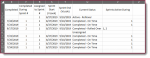
E: The date the work item item was completed
F: The sprint number the work item was completed during (sprint being a 2 week timeframe)
R: The sprint number the work item was assigned during
S: The starting date of the sprint the work item was assigned
T: The ending date of the sprint the work item was assigned
U: The current status of the work item. These are figured based off other manually entered columns, and include:
  • “Active - Current”: the item was assigned during the currently running sprint, and is still being worked on
  • “Active - Rollover”: the item was assigned during a previous sprint but not completed, and is still active in the current sprint
  • "Completed - On Time": the item was assigned and completed during the same sprint
  • "Completed - Rolled Over": the item was not completed during the same sprint it was assigned, but was completed in a later sprint
  • "Assigned - Future Sprint": the item has been assigned to a sprint that has not yet started
  • "ENTRY ERROR": the combination of data entered in the row is not complete and the correct status can’t be determined
V: This was intended to be a helper column I was going to use to list the sprints a work item was active during. If there’s a better way to accomplish my goal, this column is not needed.

The Total Summary! Tab is a synopsis page, showing various metrics pulled from the items on List!. I’m kinda stuck on one metric, the rest of the project is done. Part of the reporting needs to show various metrics as it relates only to each specific sprint. Where I am stuck is counting the items that were active during a past sprint. I am thinking I will have to use a different method of counting depending on whether the item on List! is currently active, versus whether it has been completed in the past. The trick has been how to account for items that were active over multiple sprints, then eventually completed. They need to be counted as having been active during those sprints in between when it was assigned, and when it was completed. My thought for that piece of the puzzle was to use column V to create a list of the sprint numbers the item was active during, then use FIND in the formula on Total Summary! to determine if the sprint number being reported is on the list in column V for each work item to know if that row should be counted or not. There is a limit of 5 sprints, so the formula I currently have in column V is:
=IF($F2="","",IF($F2<=$R2,$R2, IF(($F2-$R2)=1,CONCATENATE($R2,", ",$F2), IF(($F2-$R2)=2,CONCATENATE($R2,", ",$R2+1, ", ",$F2), IF(($F2-$R2)=3,CONCATENATE($R2,", ",$R2+1, ", ",$R2+2, ", ",$F2), IF(($F2-$R2)=4,CONCATENATE($R2,", ",$R2+1, ", ",$R2+2, ", ",$R2+3,$F2), IF(($F2-$R2)=5,CONCATENATE($R2,", ",$R2+1, ", ",$R2+2, ", ",$R2+3, ", ",$R2+4, ", ",$F2),"EXCEEDED MAX")))))))

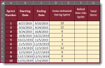
On Total Summary! (see other screenshot):
  • A: the number of the sprint being reported on in that row
  • B: the starting date of the sprint listed in A
  • C: the ending date of the sprint listed in A
  • D: new items that were assigned during the sprint number in A
  • F: this is the column I’m having trouble figuring out. It needs to count the number of work items that were active during the sprint number in A
  • G: will be D+F to get the total number of work items that were active during the sprint number in A
Hopefully this provides sufficient detail, if something doesn’t make sense, please let me know.
 

Attachments

  • 2019-11-25_11-18-23.png
    2019-11-25_11-18-23.png
    85.6 KB · Views: 9
  • 2019-11-25_11-59-20b.png
    2019-11-25_11-59-20b.png
    23.4 KB · Views: 9
Upvote 0

Forum statistics

Threads
1,214,611
Messages
6,120,510
Members
448,967
Latest member
screechyboy79

We've detected that you are using an adblocker.

We have a great community of people providing Excel help here, but the hosting costs are enormous. You can help keep this site running by allowing ads on MrExcel.com.
Allow Ads at MrExcel

Which adblocker are you using?

Disable AdBlock

Follow these easy steps to disable AdBlock

1)Click on the icon in the browser’s toolbar.
2)Click on the icon in the browser’s toolbar.
2)Click on the "Pause on this site" option.
Go back

Disable AdBlock Plus

Follow these easy steps to disable AdBlock Plus

1)Click on the icon in the browser’s toolbar.
2)Click on the toggle to disable it for "mrexcel.com".
Go back

Disable uBlock Origin

Follow these easy steps to disable uBlock Origin

1)Click on the icon in the browser’s toolbar.
2)Click on the "Power" button.
3)Click on the "Refresh" button.
Go back

Disable uBlock

Follow these easy steps to disable uBlock

1)Click on the icon in the browser’s toolbar.
2)Click on the "Power" button.
3)Click on the "Refresh" button.
Go back
Back
Top