Count unique text values based on condition in another column

[himihai]

Hello,

I need to count uniques text values in a column that contains names.
But I only need to count the unique values that are satisfying a condition in another column.

Example:

<TABLE style="WIDTH: 166pt; BORDER-COLLAPSE: collapse" cellSpacing=0 cellPadding=0 width=222 border=0><COLGROUP><COL style="WIDTH: 77pt; mso-width-source: userset; mso-width-alt: 3766" width=103><COL style="WIDTH: 89pt; mso-width-source: userset; mso-width-alt: 4352" width=119><TBODY><TR style="HEIGHT: 15pt" height=20><TD class=xl64 style="BORDER-RIGHT: windowtext 0.5pt solid; BORDER-TOP: windowtext 0.5pt solid; BORDER-LEFT: windowtext 0.5pt solid; WIDTH: 77pt; BORDER-BOTTOM: windowtext 0.5pt solid; HEIGHT: 15pt; BACKGROUND-COLOR: black" width=103 height=20>Group</TD><TD class=xl64 style="BORDER-RIGHT: windowtext 0.5pt solid; BORDER-TOP: windowtext 0.5pt solid; BORDER-LEFT: windowtext; WIDTH: 89pt; BORDER-BOTTOM: windowtext 0.5pt solid; BACKGROUND-COLOR: black" width=119>Name</TD></TR><TR style="HEIGHT: 15pt" height=20><TD class=xl63 style="BORDER-RIGHT: windowtext 0.5pt solid; BORDER-TOP: windowtext; BORDER-LEFT: windowtext 0.5pt solid; BORDER-BOTTOM: windowtext 0.5pt solid; HEIGHT: 15pt; BACKGROUND-COLOR: transparent" height=20>a</TD><TD class=xl63 style="BORDER-RIGHT: windowtext 0.5pt solid; BORDER-TOP: windowtext; BORDER-LEFT: windowtext; BORDER-BOTTOM: windowtext 0.5pt solid; BACKGROUND-COLOR: transparent">Name 1</TD></TR><TR style="HEIGHT: 15pt" height=20><TD class=xl63 style="BORDER-RIGHT: windowtext 0.5pt solid; BORDER-TOP: windowtext; BORDER-LEFT: windowtext 0.5pt solid; BORDER-BOTTOM: windowtext 0.5pt solid; HEIGHT: 15pt; BACKGROUND-COLOR: transparent" height=20>a</TD><TD class=xl63 style="BORDER-RIGHT: windowtext 0.5pt solid; BORDER-TOP: windowtext; BORDER-LEFT: windowtext; BORDER-BOTTOM: windowtext 0.5pt solid; BACKGROUND-COLOR: transparent">Name 1</TD></TR><TR style="HEIGHT: 15pt" height=20><TD class=xl63 style="BORDER-RIGHT: windowtext 0.5pt solid; BORDER-TOP: windowtext; BORDER-LEFT: windowtext 0.5pt solid; BORDER-BOTTOM: windowtext 0.5pt solid; HEIGHT: 15pt; BACKGROUND-COLOR: transparent" height=20>a</TD><TD class=xl63 style="BORDER-RIGHT: windowtext 0.5pt solid; BORDER-TOP: windowtext; BORDER-LEFT: windowtext; BORDER-BOTTOM: windowtext 0.5pt solid; BACKGROUND-COLOR: transparent">Name 2</TD></TR><TR style="HEIGHT: 15pt" height=20><TD class=xl63 style="BORDER-RIGHT: windowtext 0.5pt solid; BORDER-TOP: windowtext; BORDER-LEFT: windowtext 0.5pt solid; BORDER-BOTTOM: windowtext 0.5pt solid; HEIGHT: 15pt; BACKGROUND-COLOR: transparent" height=20>a</TD><TD class=xl63 style="BORDER-RIGHT: windowtext 0.5pt solid; BORDER-TOP: windowtext; BORDER-LEFT: windowtext; BORDER-BOTTOM: windowtext 0.5pt solid; BACKGROUND-COLOR: transparent">Name 2</TD></TR><TR style="HEIGHT: 15pt" height=20><TD class=xl63 style="BORDER-RIGHT: windowtext 0.5pt solid; BORDER-TOP: windowtext; BORDER-LEFT: windowtext 0.5pt solid; BORDER-BOTTOM: windowtext 0.5pt solid; HEIGHT: 15pt; BACKGROUND-COLOR: transparent" height=20>b</TD><TD class=xl63 style="BORDER-RIGHT: windowtext 0.5pt solid; BORDER-TOP: windowtext; BORDER-LEFT: windowtext; BORDER-BOTTOM: windowtext 0.5pt solid; BACKGROUND-COLOR: transparent">Name 1</TD></TR><TR style="HEIGHT: 15pt" height=20><TD class=xl63 style="BORDER-RIGHT: windowtext 0.5pt solid; BORDER-TOP: windowtext; BORDER-LEFT: windowtext 0.5pt solid; BORDER-BOTTOM: windowtext 0.5pt solid; HEIGHT: 15pt; BACKGROUND-COLOR: transparent" height=20>b</TD><TD class=xl63 style="BORDER-RIGHT: windowtext 0.5pt solid; BORDER-TOP: windowtext; BORDER-LEFT: windowtext; BORDER-BOTTOM: windowtext 0.5pt solid; BACKGROUND-COLOR: transparent">Name 2</TD></TR><TR style="HEIGHT: 15pt" height=20><TD class=xl63 style="BORDER-RIGHT: windowtext 0.5pt solid; BORDER-TOP: windowtext; BORDER-LEFT: windowtext 0.5pt solid; BORDER-BOTTOM: windowtext 0.5pt solid; HEIGHT: 15pt; BACKGROUND-COLOR: transparent" height=20>b</TD><TD class=xl63 style="BORDER-RIGHT: windowtext 0.5pt solid; BORDER-TOP: windowtext; BORDER-LEFT: windowtext; BORDER-BOTTOM: windowtext 0.5pt solid; BACKGROUND-COLOR: transparent">Name 3</TD></TR><TR style="HEIGHT: 15pt" height=20><TD class=xl63 style="BORDER-RIGHT: windowtext 0.5pt solid; BORDER-TOP: windowtext; BORDER-LEFT: windowtext 0.5pt solid; BORDER-BOTTOM: windowtext 0.5pt solid; HEIGHT: 15pt; BACKGROUND-COLOR: transparent" height=20>c</TD><TD class=xl63 style="BORDER-RIGHT: windowtext 0.5pt solid; BORDER-TOP: windowtext; BORDER-LEFT: windowtext; BORDER-BOTTOM: windowtext 0.5pt solid; BACKGROUND-COLOR: transparent">Name 4</TD></TR></TBODY></TABLE>

So I need to count unique names from group "a"

I already got the formula for counting the unique values from the whole list, and I just need to add the condition that would restrict the search only to one group (condition).

Any ideas?

 

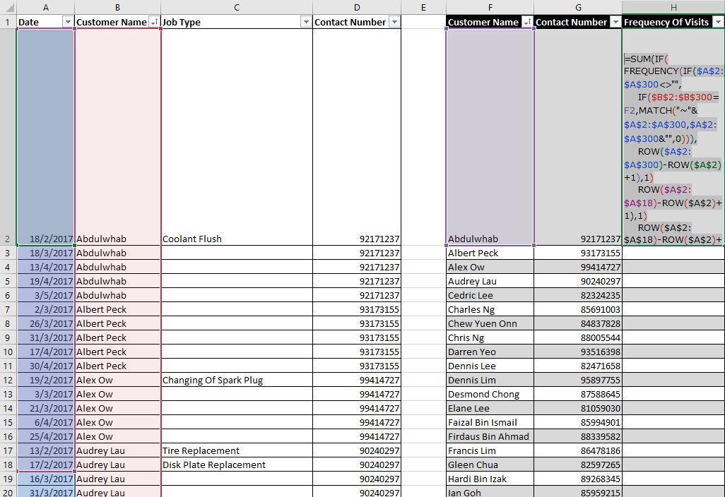[Aladin Akyurek]

...any idea what I am doing wrong?

Keep changing the ranges involved and we won't get anywhere...

What is the sheet name where the data is located?

What are the current ranges and what kind of data do they house?

 

[akshatku]

Keep changing the ranges involved and we won't get anywhere...

What is the sheet name where the data is located?

What are the current ranges and what kind of data do they house?

So the data is like the one shown below:

Agency	Participating
NUM	Y
SIP	Y
HUN	Y
GUY	N
POE	Y
OIN	N
POE	Y
HUN	Y
HBN	Y
HAJ	N
PIN	N

<colgroup><col><col></colgroup><tbody>
</tbody>

I need to find the number of unique participating agencies (for which Participating=Y) excluding the agencies POE and HUN.
How I would do it manually is- I first filter out to remove the agencies POE and HUN. Then I filter out to include only "Y" in the Participating Column. Then I would remove duplicates from the resulting Agency column to give me the answer. Is there a formula to do the same? Please note that there are more than 1000 agencies in actual data and I need to exclude 3 agencies from them.

Please let me know.

 

[Aladin Akyurek]

Let A1:B12 house the data.

Control+shift+enter, not just enter:

=SUM(IF(FREQUENCY(IF(1-(A2:A12=""),IF(B2:B12="Y",IF(1-ISNUMBER(MATCH(A2:A12,{"POE","HUN"},0)),MATCH(A2:A12,A2:A12,0)))),ROW(A2:A12)-ROW(A2)+1),1))

 

[mjm65]

Aladin,

I have a similar question as above, but I believe a bit simpler. ZI need to count the number of unique names that meet the second condition, both text:


Name1 PASS
Name1 PASS
Name1 FAIL
Name2 PASS
Name2 FAIL
etc.

I want to look at those the "PASS" and then count the number of unique names from the first column.

For the example above, it should return 2.

 

[Aladin Akyurek]

@mjm65

Control+shift+enter, not just enter:

=SUM(IF(FREQUENCY(IF(1-(A2:A6=""),IF(B2:B6="PASS",MATCH(A2:A6,A2:A6,0))),ROW(A2:A6)-ROW(A2)+1),1))

 

[mjm65]

@mjm65

Control+shift+enter, not just enter:

=SUM(IF(FREQUENCY(IF(1-(A2:A6=""),IF(B2:B6="PASS",MATCH(A2:A6,A2:A6,0))),ROW(A2:A6)-ROW(A2)+1),1))

Thanks a bunch. It's working now!

 

[Aladin Akyurek]

Thanks a bunch. It's working now!

You are welcome.

 

[KurouTendou]

Hi, So I'm trying to count the number of unique occurrences of a date based on the customer name in my table. I found and tried modifying a formula i found on an earlier page in this thread but when I try to ctrl-shift-enter it Excel tells me that my formula is wrong. Can anyone tell me what my error is or suggest a better formula for me? The table looks like this currently,
<blockquote class="imgur-embed-pub" lang="en" data-id="a/PtyUn"><a href="//imgur.com/PtyUn"></a></blockquote>******** async src="//s.imgur.com/min/embed.js" charset="utf-8">*********>
and the formula I'm using is : =SUM(IF(FREQUENCY(IF($A$2:$A$300<>"", IF($B$2:$B$300=F2,MATCH("~"&$A$2:$A$300,$A$2:$A$300&"",0))),
ROW($A$2:$A$300)-ROW($A$2)+1),1)
ROW($A$2:$A$300)-ROW($A$2)+1),1)
ROW($A$2:$A$300)-ROW($A$2)+1),1)

 

[KurouTendou]

Hi, So I'm trying to count the number of unique occurrences of a date based on the customer name in my table. I found and tried modifying a formula i found on an earlier page in this thread but when I try to ctrl-shift-enter it Excel tells me that my formula is wrong. Can anyone tell me what my error is or suggest a better formula for me? The table looks like this currently,******** async src="//s.imgur.com/min/embed.js" charset="utf-8">*********>and the formula I'm using is : =SUM(IF(FREQUENCY(IF($A$2:$A$300<>"", IF($B$2:$B$300=F2,MATCH("~"&$A$2:$A$300,$A$2:$A$300&"",0))), ROW($A$2:$A$300)-ROW($A$2)+1),1) ROW($A$2:$A$300)-ROW($A$2)+1),1) ROW($A$2:$A$300)-ROW($A$2)+1),1)

Sorry I screwed up posting the picture. It looks like this :

 

[Aladin Akyurek]

Hi, So I'm trying to count the number of unique occurrences of a date based on the customer name in my table. I found and tried modifying a formula i found on an earlier page in this thread but when I try to ctrl-shift-enter it Excel tells me that my formula is wrong. Can anyone tell me what my error is or suggest a better formula for me? The table looks like this currently,

​

******** async src="//s.imgur.com/min/embed.js" charset="utf-8">*********>
and the formula I'm using is : =SUM(IF(FREQUENCY(IF($A$2:$A$300<>"", IF($B$2:$B$300=F2,MATCH("~"&$A$2:$A$300,$A$2:$A$300&"",0))),
ROW($A$2:$A$300)-ROW($A$2)+1),1)
ROW($A$2:$A$300)-ROW($A$2)+1),1)
ROW($A$2:$A$300)-ROW($A$2)+1),1)

Control+shift+enter, not just enter:

=SUM(IF(FREQUENCY(IF($A$2:$A$300<>"", IF($B$2:$B$300=F2,MATCH("~"&$A$2:$A$300,$A$2:$A$300&"",0))),ROW($A$2:$A$300)-ROW($A$2)+1),1))​