Getting value on Y axis by putting X axis value

[kashifjillani]

Hello to all the experts of Excel,

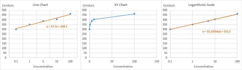
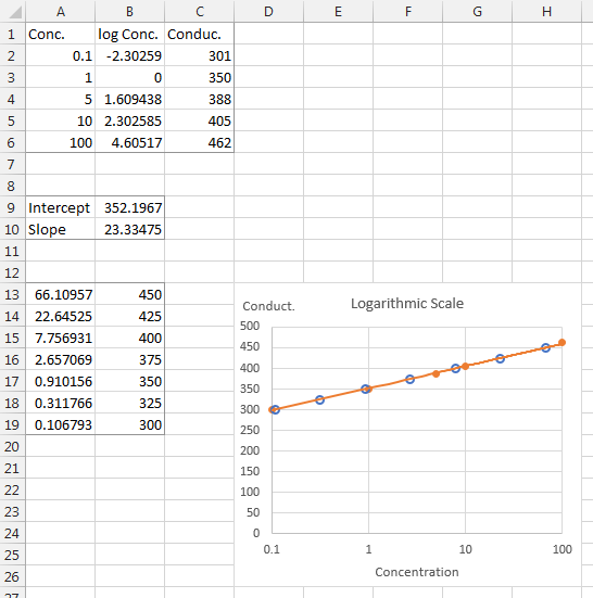
I still can not figure out the way to get the values in a chart/graph by putting an specific X axis value.

e.g.

There is relation between Gauge height and Flow

<TABLE style="WIDTH: 96pt; BORDER-COLLAPSE: collapse" border=0 cellSpacing=0 cellPadding=0 width=128><COLGROUP><COL style="WIDTH: 48pt" span=2 width=64><TBODY><TR style="HEIGHT: 15pt" height=20><TD style="BORDER-BOTTOM: #f0f0f0; BORDER-LEFT: #f0f0f0; BACKGROUND-COLOR: transparent; WIDTH: 48pt; HEIGHT: 15pt; BORDER-TOP: #f0f0f0; BORDER-RIGHT: #f0f0f0" height=20 width=64>Gauge</TD><TD style="BORDER-BOTTOM: #f0f0f0; BORDER-LEFT: #f0f0f0; BACKGROUND-COLOR: transparent; WIDTH: 48pt; BORDER-TOP: #f0f0f0; BORDER-RIGHT: #f0f0f0" width=64>Flow </TD></TR><TR style="HEIGHT: 15pt" height=20><TD style="BORDER-BOTTOM: #f0f0f0; BORDER-LEFT: #f0f0f0; BACKGROUND-COLOR: transparent; HEIGHT: 15pt; BORDER-TOP: #f0f0f0; BORDER-RIGHT: #f0f0f0" height=20 align=right>0.305</TD><TD style="BORDER-BOTTOM: #f0f0f0; BORDER-LEFT: #f0f0f0; BACKGROUND-COLOR: transparent; BORDER-TOP: #f0f0f0; BORDER-RIGHT: #f0f0f0" align=right>0</TD></TR><TR style="HEIGHT: 15pt" height=20><TD style="BORDER-BOTTOM: #f0f0f0; BORDER-LEFT: #f0f0f0; BACKGROUND-COLOR: transparent; HEIGHT: 15pt; BORDER-TOP: #f0f0f0; BORDER-RIGHT: #f0f0f0" height=20 align=right>0.32</TD><TD style="BORDER-BOTTOM: #f0f0f0; BORDER-LEFT: #f0f0f0; BACKGROUND-COLOR: transparent; BORDER-TOP: #f0f0f0; BORDER-RIGHT: #f0f0f0" align=right>0.10022</TD></TR><TR style="HEIGHT: 15pt" height=20><TD style="BORDER-BOTTOM: #f0f0f0; BORDER-LEFT: #f0f0f0; BACKGROUND-COLOR: transparent; HEIGHT: 15pt; BORDER-TOP: #f0f0f0; BORDER-RIGHT: #f0f0f0" height=20 align=right>0.341388</TD><TD style="BORDER-BOTTOM: #f0f0f0; BORDER-LEFT: #f0f0f0; BACKGROUND-COLOR: transparent; BORDER-TOP: #f0f0f0; BORDER-RIGHT: #f0f0f0" align=right>0.27539</TD></TR><TR style="HEIGHT: 15pt" height=20><TD style="BORDER-BOTTOM: #f0f0f0; BORDER-LEFT: #f0f0f0; BACKGROUND-COLOR: transparent; HEIGHT: 15pt; BORDER-TOP: #f0f0f0; BORDER-RIGHT: #f0f0f0" height=20 align=right>0.381347</TD><TD style="BORDER-BOTTOM: #f0f0f0; BORDER-LEFT: #f0f0f0; BACKGROUND-COLOR: transparent; BORDER-TOP: #f0f0f0; BORDER-RIGHT: #f0f0f0" align=right>0.85528</TD></TR><TR style="HEIGHT: 15pt" height=20><TD style="BORDER-BOTTOM: #f0f0f0; BORDER-LEFT: #f0f0f0; BACKGROUND-COLOR: transparent; HEIGHT: 15pt; BORDER-TOP: #f0f0f0; BORDER-RIGHT: #f0f0f0" height=20 align=right>0.401708</TD><TD style="BORDER-BOTTOM: #f0f0f0; BORDER-LEFT: #f0f0f0; BACKGROUND-COLOR: transparent; BORDER-TOP: #f0f0f0; BORDER-RIGHT: #f0f0f0" align=right>1.32224</TD></TR><TR style="HEIGHT: 15pt" height=20><TD style="BORDER-BOTTOM: #f0f0f0; BORDER-LEFT: #f0f0f0; BACKGROUND-COLOR: transparent; HEIGHT: 15pt; BORDER-TOP: #f0f0f0; BORDER-RIGHT: #f0f0f0" height=20 align=right>0.413752</TD><TD style="BORDER-BOTTOM: #f0f0f0; BORDER-LEFT: #f0f0f0; BACKGROUND-COLOR: transparent; BORDER-TOP: #f0f0f0; BORDER-RIGHT: #f0f0f0" align=right>1.69248</TD></TR><TR style="HEIGHT: 15pt" height=20><TD style="BORDER-BOTTOM: #f0f0f0; BORDER-LEFT: #f0f0f0; BACKGROUND-COLOR: transparent; HEIGHT: 15pt; BORDER-TOP: #f0f0f0; BORDER-RIGHT: #f0f0f0" height=20 align=right>0.433354</TD><TD style="BORDER-BOTTOM: #f0f0f0; BORDER-LEFT: #f0f0f0; BACKGROUND-COLOR: transparent; BORDER-TOP: #f0f0f0; BORDER-RIGHT: #f0f0f0" align=right>2.46828</TD></TR><TR style="HEIGHT: 15pt" height=20><TD style="BORDER-BOTTOM: #f0f0f0; BORDER-LEFT: #f0f0f0; BACKGROUND-COLOR: transparent; HEIGHT: 15pt; BORDER-TOP: #f0f0f0; BORDER-RIGHT: #f0f0f0" height=20 align=right>0.452996</TD><TD style="BORDER-BOTTOM: #f0f0f0; BORDER-LEFT: #f0f0f0; BACKGROUND-COLOR: transparent; BORDER-TOP: #f0f0f0; BORDER-RIGHT: #f0f0f0" align=right>3.43106</TD></TR><TR style="HEIGHT: 15pt" height=20><TD style="BORDER-BOTTOM: #f0f0f0; BORDER-LEFT: #f0f0f0; BACKGROUND-COLOR: transparent; HEIGHT: 15pt; BORDER-TOP: #f0f0f0; BORDER-RIGHT: #f0f0f0" height=20 align=right>0.482379</TD><TD style="BORDER-BOTTOM: #f0f0f0; BORDER-LEFT: #f0f0f0; BACKGROUND-COLOR: transparent; BORDER-TOP: #f0f0f0; BORDER-RIGHT: #f0f0f0" align=right>5.3022</TD></TR><TR style="HEIGHT: 15pt" height=20><TD style="BORDER-BOTTOM: #f0f0f0; BORDER-LEFT: #f0f0f0; BACKGROUND-COLOR: transparent; HEIGHT: 15pt; BORDER-TOP: #f0f0f0; BORDER-RIGHT: #f0f0f0" height=20 align=right>0.511557</TD><TD style="BORDER-BOTTOM: #f0f0f0; BORDER-LEFT: #f0f0f0; BACKGROUND-COLOR: transparent; BORDER-TOP: #f0f0f0; BORDER-RIGHT: #f0f0f0" align=right>7.77429</TD></TR><TR style="HEIGHT: 15pt" height=20><TD style="BORDER-BOTTOM: #f0f0f0; BORDER-LEFT: #f0f0f0; BACKGROUND-COLOR: transparent; HEIGHT: 15pt; BORDER-TOP: #f0f0f0; BORDER-RIGHT: #f0f0f0" height=20 align=right>0.522962</TD><TD style="BORDER-BOTTOM: #f0f0f0; BORDER-LEFT: #f0f0f0; BACKGROUND-COLOR: transparent; BORDER-TOP: #f0f0f0; BORDER-RIGHT: #f0f0f0" align=right>8.9451</TD></TR><TR style="HEIGHT: 15pt" height=20><TD style="BORDER-BOTTOM: #f0f0f0; BORDER-LEFT: #f0f0f0; BACKGROUND-COLOR: transparent; HEIGHT: 15pt; BORDER-TOP: #f0f0f0; BORDER-RIGHT: #f0f0f0" height=20 align=right>0.561209</TD><TD style="BORDER-BOTTOM: #f0f0f0; BORDER-LEFT: #f0f0f0; BACKGROUND-COLOR: transparent; BORDER-TOP: #f0f0f0; BORDER-RIGHT: #f0f0f0" align=right>13.53592</TD></TR><TR style="HEIGHT: 15pt" height=20><TD style="BORDER-BOTTOM: #f0f0f0; BORDER-LEFT: #f0f0f0; BACKGROUND-COLOR: transparent; HEIGHT: 15pt; BORDER-TOP: #f0f0f0; BORDER-RIGHT: #f0f0f0" height=20 align=right>0.589</TD><TD style="BORDER-BOTTOM: #f0f0f0; BORDER-LEFT: #f0f0f0; BACKGROUND-COLOR: transparent; BORDER-TOP: #f0f0f0; BORDER-RIGHT: #f0f0f0" align=right>17.68</TD></TR></TBODY></TABLE>


If I draw the curve with Flow on X-axis and Gage on Y-axis and then want to know the flow at Gage 0.53m.

OR

By putting flow value to know Gage height.

Regards,

 

[jimmyeatstage]

Jon,

I tried reading your answers to previous questions on this thread and it is very hard for me to follow but I don't think they apply to me. I have a marked scatter plot with the following data. How will I find an x value by inputting a y value?

Discharge (cm3/s) (x)	Valve setting
0	-90
4.864	-64
20.066	-56
36.483	-54
58.373	-44
121.61	-31
167.822	0
220.114	32
322.672	48
421.581	63
454.272	90

<colgroup><col><col></colgroup><tbody>
</tbody>

 

[jimmyeatstage]

Oops. Meant to ask this: How will I find a y value by inputting an x value?

Discharge (cm3/s)	Valve setting (x)
0	-90
4.864	-64
20.066	-56
36.483	-54
58.373	-44
121.61	-31
167.822	0
220.114	32
322.672	48
421.581	63
454.272	90

<tbody>
</tbody>

[/QUOTE]

 

[Jon Peltier]

The original post said it wanted to find Y for an input X value, but in the description the opposite was requested.

You should be able to modify my approach to actually input X and get Y.

 

[Savagefool]

So I was wondering if I could do the same, my data is like this:

Tidal Time	Tidal Height
01:00
02:00
03:00
04:00
05:00	5
06:00
07:00
08:00
09:00
10:00
11:00	1.2
12:00
13:00
14:00
15:00
16:00
17:00	5.2
18:00
19:00
20:00
21:00
22:00
23:00	1.1
00:00

<tbody>
</tbody>

Note that the other values are not known, thus when I put in Y i need to get X based on the line that connects the two, any help would be appreciated. Thank you in advance!

 

[Jon Peltier]

You can use the same approach. Starting with your data:

Note that I've used date-time values in the first column, not just times, because date-times will continue to increase monotonically even after midnight.

The top chart shows your tide extrema. The middle chart shows a linear interpolation from a peak to a valley or vice versa. The bottom chart shows behavior that's closer to real tides, that is, more of a sinusoidal rise and fall. Not exactly, because of currents and geographical irregularities, but the sine wave is closer than the sawtooth in the middle chart.

The linear interpolation formula in C2 is
=(A3-A$2)/(A$8-A$2)*(B$8-B$2)+B$2

This is filled down to C7, then copied again to C9, where the fixed points are adjusted to
=(A9-A$8)/(A$14-A$8)*(B$14-B$8)+B$8

etc.

The trigonometric interpolation formula in D2 is
=(B$2+B$8)/2+COS((A3-A$2)/(A$8-A$2)*PI())*(B$2-B$8)/2

This is filled down to D7, and copied into D9 where it's adjusted to
=(B$8+B$14)/2+COS((A9-A$8)/(A$14-A$8)*PI())*(B$8-B$14)/2

etc.

But this isn't easy enough to use yet, since you need to manually enter the interpolation formulas into column C or D.

Here I've entered tide data for Dennisport MA into columns A and B. This is a lot closer to the data you can get from the web. I'm going to plot hourly interpolated tide heights for 8/19 noon to 8/20 noon (linear) and 8/20-8/21 midnight to 8/21-8/22 midnight (trigonometric).

Cell D2 has this formula (filled down to D26):
=MATCH(E2,$A$2:$A$15)

Cell F2 has this linear interpolation formula (filled down to F26):
=(E2-INDEX($A$2:$A$15,D2))/(INDEX($A$2:$A$15,D2+1)-INDEX($A$2:$A$15,D2))
*(INDEX($B$2:$B$15,D2+1)-INDEX($B$2:$B$15,D2))+INDEX($B$2:$B$15,D2)

Cell H2 has this formula (filled down to H26):
=MATCH(I2,$A$2:$A$15)

Cell J2 has this linear interpolation formula (filled down to J26):
=COS((I2-INDEX($A$2:$A$15,H2))/(INDEX($A$2:$A$15,H2+1)-INDEX($A$2:$A$15,H2))*PI())
*(INDEX($B$2:$B$15,H2)-INDEX($B$2:$B$15,H2+1))/2+(INDEX($B$2:$B$15,H2)+INDEX($B$2:$B$15,H2+1))/2

You can see how well the points fit with the input tide data:

 

[Aventus]

Mine is similar question.

I've been given a graph and equation of y=37.7x +268.1 has been provided. I need to find out the concentration from given conductivity. The graph has been produced using the following data:


X-axis (concentration) <--------> Y-axis (conductivity)
0.1 <--------------------------------->301
1 <--------------------------------->350
5 <--------------------------------> 388
10 <--------------------------------> 405



I have conductivity readings for 80 samples, how can I find out the concentration for them using the above formula.

Thanks in advance

 

[Jon Peltier]

Your equation is not a good fit for the limited data you've shown.

Are you trying to fit a number of conductivity readings between your data's min and max conductivity to get new concentration readings between the min and max concentration? Then follow the procedure given above. If you can't get it, show us how far you got and where you got stuck.

 

[Aventus]

That's the graph that I've been provided with. I'm trying to get new concentration readings for the samples I've collected. There are three conductivity values for each sample (control, boiling and filtration) and I need to find out the concentration for each conductivity value.

 

[Jon Peltier]

Don't ever calculate a trendline on a line chart. Notice how the X axis spacing is not proportional to the values of the labels?

Convert the chart to an XY chart. Then use a log scale for the X axis. This produces a perfectly straight line.

Left: line chart points (blue) and trendline (orange). Middle: Scatter chart points and line (blue). Right: logarithmic scatter plot points (blue) and trendline (orange).

The trendline formula is of the form Y = A ln(x) + B

You can calculate A and B easily enough. Here's the data:

I've inserted a column for the log of the concentration. The formula in B2 (filled down to B6) is

=LN(A2)

The calculation for A in cell B10 is

=SLOPE(C2:C6,B2:B6)

and for B in cell B9 is

=INTERCEPT(C2:C6,B2:B6)

We can invert the formula above

Conductivity = A ln(Concentration) + B

into this

Concentration = exp((Conductivity - B)/A)

I use this to calculate the concentrations in A13:A19 from the conductivities in B13:B19. The formula in cell A13, filled down to A19, is

=EXP((B13-$B$9)/$B$10)

I've plotted this as blue unfilled circles on the log plot, where the trendline and the original points are orange.

 

[Aventus]

I can't thank you enough Jon Peltier.