Excel Chart from variable data to ignore zero in 1 column

[jonto81]

Hi,

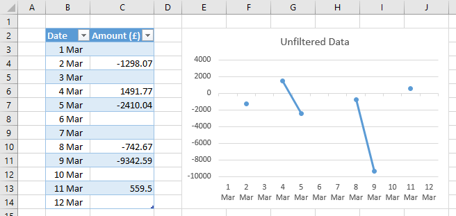
I am trying to get data to plot in a chart which is taken from a Vlookup on the date, so only some of the dates have data beside them, others have #N/A (can change this to whatever I want).

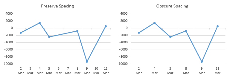
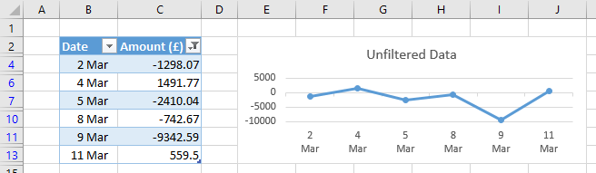
My aim is to produce a Bar chart that only shows the dates that have any data - for example my graph I envisage as below:


5
4
3
2
1
02/03/15 04/03/15 15/03/15 16/03/15 31/03/15


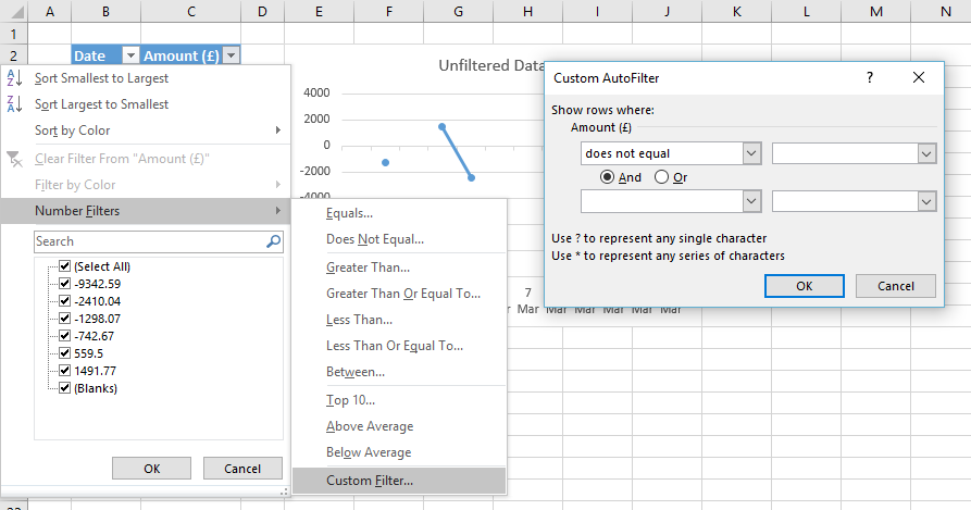
currently I get every date of the month along the X axis due to my column having each date listed even if the value is zero, can anyone suggest a way to fix this without having to amend the source data?

Thanks

J

 

[Jon Peltier]

My tutorial Dynamic Charts explains how to define Names based on whether cells contain numbers, and how to use these Names to create dynamic charts.

 

[jonto81]

Hi

I have had a look at this and it works for removing blank values from the end, however I also have blank values in the middle of my data set I need removed from the charting:

Date	Amount (£)
01/03/16
02/03/16	-1298.07
03/03/16
04/03/16	1491.77
05/03/16	-2410.04
06/03/16
07/03/16
08/03/16	-742.67
09/03/16	-9342.59
10/03/16
11/03/16	559.5
12/03/16

<colgroup><col><col></colgroup><tbody>
</tbody>

have you any suggestions?

 

[Jon Peltier]

What kind of chart? Do you want all dates to appear on the axis, so the spacing is apparent, or do you want only the dates that have a corresponding amount, with spacing independent of elapsed time?

 

[jonto81]

Hi,

I am only looking for the dates that have a corresponding amount - I can't

 

[Jon Peltier]

Here's your data and a line chart. I've selected the data and pressed Ctrl+T to convert it to a Table, which is a powerful data feature in Excel.

Here's how to apply a filter to the data. Click the dropdown on the Amount column header. Click Number Filters, then Custom Filter, then find "does not equal" in the left dropdown of the Custom AutoFilter dialog (I suppose you could have just selected Does Not Equal in the pop-up menu), and keep the second dropdown blank.

Here's the table and chart with filtered data. Note that rows are hidden. By default, charts do not show data from hidden cells. Note also that charts resize when rows and columns under them are resized, so the chart has shrunk. You need to resize the chart. (You could have formatted the Chart Area of the chart, and changed the Properties so it moves but doesn't resize with cells.)