DAX RankX() - Blank and ignore filter context

[potap]

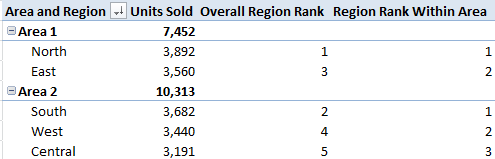
I have a pivot table where I want to rank the overall performance of regions by clearing the area filter.

It looks just like this example :

https://powerpivotpro.com/2015/06/rankx-apalooza-within-and-across-groups-with-filters-etc/

I first wrote a measure similar to this one :

=
IF (
HASONEVALUE ( Stores[Region] ),
RANKX (
ALL ( Stores[Region] ),
CALCULATE ( [Units Sold], ALL ( Stores[Area] ) ),
,
1,
SKIP
),
BLANK ()
)

I understand it and if a region doesn't have any unit sold (blank result), it will be ranked as number 1. I want the first non blank to be ranked as number 1.

I tried this version and now I don't rank blank values but I don't remove the Area filter within the rank. My results are similar to the ''Region Rank Within Area'' measure in the image above.

=
IF (
HASONEVALUE ( Stores[Region] ),
RANKX (
FILTER ( ALL ( Stores[Region] ), NOT ( ISBLANK ( [Units Sold] ) ) ),
CALCULATE ( [Units Sold], ALL ( Stores[Area] ) ),
,
1,
SKIP
),
BLANK ()
)

How can I rank my regions that have at least 1 unit sold and ignore the area filter in my pivot table at the same time?

Thank you!

 

[potap]

Here is a file that shows what I mean.

https://drive.google.com/file/d/0BxcndF-RTt_oY2lHSzdRSVlaMmM/view?usp=sharing

 

[Ozeroth]

Hi potap,

You're on the right track here.
Your measure needs to do two things:

1. Return BLANK for Regions where Units Sold = BLANK
2. Within RANKX, only iterate over Regions with sales (i.e. Units Sold <> BLANK)

Here is a potential measure that does this and works in the PivotTable you provided. It may need tweaking to handle all possible filter situations:

=
IF (
    AND ( HASONEVALUE ( Stores[Region] ), [COLOR=#ff0000][B]NOT ( ISBLANK ( [Units Sold] ) )[/B][/COLOR] ),
    RANKX (
        [B][COLOR=#008000]CALCULATETABLE ( SUMMARIZE ( Sales, Stores[Region] ), ALLSELECTED ( Stores ) )[/COLOR][/B],
        CALCULATE ( [Units Sold], ALL ( Stores[Area] ) ),
        ,
        1,
        SKIP
    ),
    BLANK ()
)

1. The code in red performs the first check
2. The code in green is one way of creating a list of Regions that actually have sales, and are not excluded by filters on Stores in the overall PivotTable. It is necessary to clear filters on both Stores[Area] and Stores[Region].
   ALLSELECTED could be changed to ALL if you wanted the rank to be evaluated relative to all regions even if they are filtered out in the PivotTable.
   You could also use FILTER like your example, with an alternate green expression like:
   CALCULATETABLE ( FILTER ( VALUES(Stores[Region] ), NOT ( ISBLANK ( [Units Sold] ) ) ), ALLSELECTED ( Stores ) )

Anyway, have a play with that and see if it works for you.

Regards,
Owen

 

[potap]

Thanks a lot, solved my problem!