Allocate costs on a monthly basis

[Exelance]

Hi all,

I tried looking for an answer myself (or here), but I just can't get it to work.
Hopefully the answer is understandeable for a non-IT guy (finance background)...

So the problem:

We have about 100 employees working on our payroll and we want to allocate their individual cost to 4 different business units.
It's possible that person A works from januari - march on business unit 1 and from then on business unit 2.

So basically, we have 1 large table as follows:

We are updating this table as soon as there is a change in the budget/forecast where this person will work.
I already unpivoted that table to the format below:

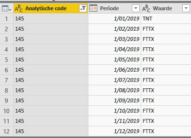
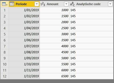
Next to that, I have a datatable with the same employee numbers and their cost per month (below dummy values).

So the end result would have to be that I know, for each business unit, what my payroll cost was in each month.
Every month, the new actual payroll cost will be added to the model.

In the above example, the cost of employee 145 should be added in business unit TNT in January and as of February it should be allocated to FTTX.

I hope my problem makes sense?
What is the best practice to solve this, as I don't believe I'm the only one with this request...

Thanks a lot for helping me out!

 

[Col Delane]

Howdy

Sorry about the way the tables appear - I can't get the sheet uploading tools to work properly.

If I understand your explanation correctly:

1. You really have two source data tables:
   1. Employee code x month x allocated business unit (There's an assumption here that each employee is allocated 100% to a business in each month, rather than being split between more than one unit)
   2. Employee code x month x monthly payroll cost
2. Your ultimate objective is to calculate the monthly payroll cost for each business unit.

If the above is correct, then I think the solution is relatively simple.

1. I would lay out the employee cost table (#1.2 above) in the same way as the Employee code x month x allocated business unit table (#1.1 above) shown in your post.
2. These two tables should then have exactly the same dimensions - except for the total row.

Below are sample tables using some sample data to demonstrate:
Table 1 (A1:M4)
Table 2 (A6:M10)

Employee	Jan-19	Feb-19	Mar-19	Apr-19	May-19	Jun-19	Jul-19	Aug-19	Sep-19	Oct-19	Nov-19	Dec-19
143	TNT	TNT	TNT	TNT	TNT	TNT	TNT	TNT	TNT	TNT	TNT	TNT
144	TNT	TNT	TNT	TNT	TNT	TNT	TNT	TNT	TNT	TNT	TNT	TNT
145	TNT	FTTX	FTTX	FTTX	FTTX	FTTX	FTTX	FTTX	FTTX	FTTX	FTTX	FTTX
Employee	Jan -19	Feb-19	Mar-19	Apr-19	May-19	Jun-19	Jul-19	Aug-19	Sep-19	Oct-19	Nov-19	Dec-19
143	1,000	1,500	2,000	2,500	3,000	3,500	4,000	4,500	5,000	5,500	6,000	6,500
144	1,000	1,500	2,000	2,500	3,000	3,500	4,000	4,500	5,000	5,500	6,000	6,500
145	1,000	1,500	2,000	2,500	3,000	3,500	4,000	4,500	5,000	5,500	6,000	6,500
Total	3,000	4,500	6,000	7,500	9,000	10,500	12,000	13,500	15,000	16,500	18,000	19,500

<tbody>
</tbody>

The final result table (business unit x month x total payroll cost) should also be laid in a similar fashion (business units down the LHS and months across the top).
Table 3 (A13:M16)

Unit	Jan-19	Feb-19	Mar-19	Apr-19	May-19	Jun-19	Jul-19	Aug-19	Sep-19	Oct-19	Nov-19	Dec-19
TNT	3,000	3,000	4,000	5,000	6,000	7,000	8,000	9,000	10,000	11,000	12,000	13,000
FTTX	-	1,500	2,000	2,500	3,000	3,500	4,000	4,500	5,000	5,500	6,000	6,500
Total	3,000	4,500	6,000	7,500	9,000	10,500	12,000	13,500	15,000	16,500	18,000	19,500

<tbody>
</tbody>

The formula at the intersection of business unit code x month is like this:
TNT x Jan-19 (B14) = SUMPRODUCT( ( B$2:B$4 = $A14 ) * ( B$7:B$9 ) )
FTTX x Jan-19 (B15) = SUMPRODUCT( ( B$2:B$4 = $A15 ) * ( B$7:B$9 ) )

(These formula should be using structured references as they reference tables but for some unknown reason my XL2007 is misbehaving!)

Does this do what you're seeking?

 

[Exelance]

Does this do what you're seeking?

Thanks for your reply!

Is it correct to assume that this only works when the order of both tables are the same and both have equal number of rows?
For example: we sometimes have independents working for us but they don't always work fulltime. So it could happen that one month, they have no cost.
So this means that there are less rows in the cost table compared to the budget table with the business unit allocation.

Is there no function in Power BI (preferably) or PowerQuery/Pivot to look up the value based on a relationship between both tables (being the employee number) and on a monthly base?

The result in words should be like:

Person A had a cost of 1K this month, so let's see in which business unit he worked this month so we can add it to that business unit.
In my head it seems so simple

 

[Exelance]

I can't seem to edit my post so sorry for the double..

But I think I figured it out.

I created in both tables a new column which is a concatinate of employee&period (e.g. 1451/01/2019).
Then I merged both tables in power bi based on the concatinated columns.

Seems to do what I intended to achieve!

 

[Col Delane]

Is it correct to assume that this only works when the order of both tables are the same and both have equal number of rows?
For example: we sometimes have independents working for us but they don't always work fulltime. So it could happen that one month, they have no cost.
So this means that there are less rows in the cost table compared to the budget table with the business unit allocation.

As I suggested, why not lay out the employee monthly cost table the same way as the employee x business unit table (i.e. with months across the page rather than down)? This way the No. of columns will always be the same, so you just need a row in both source data tables for every employee. Either way, you can have a month with zero cost for an employee which any calculation using that value will also return as zero.

Is there no function in Power BI (preferably) or PowerQuery/Pivot to look up the value based on a relationship between both tables (being the employee number) and on a monthly base?

The result in words should be like:
Person A had a cost of 1K this month, so let's see in which business unit he worked this month so we can add it to that business unit.
In my head it seems so simple

I am yet to come to grips with PBI, PQ & PP so can't answer that question - but I don't think you need that level of functionality to achieve the outcome you're seeking.

What you're describing is kind of what SUMPRODUCT is doing, but if you have the months across the page rather than down, and in the same columns in all tables, you don't need to bother about the relationship between employee and month as the months are always in the same column as the calculating formula.
As an alternative, because the monthly cost of each employee is allocated 100% to the business unit (no apportionment required), there is actually no multiplication involved but really an addition. As such, you can also use the SUMIFS function in place of SUMPRODUCT (provided the row dimensions of both source tables are the same), viz:
= SUMIFS( B$7:B$9, B$2:B$4, $A14 )