Cash flow in Power Pivot and using DAX

[didijaba]

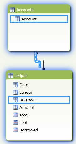
Hello, I would like to show cash flow for lending and borrowing (landing as + and borrowing as -) using Power Pivot and DAX. First table is what I have, and second is what I want. Do you have any ideas how to do this?

<style type="text/css">
table.tableizer-table {
border: 1px solid #CCC; font-family: Arial, Helvetica, sans-serif
font-size: 12px;
}
.tableizer-table td {
padding: 4px;
margin: 3px;
border: 1px solid #ccc;
}
.tableizer-table th {
background-color: #104E8B;
color: #FFF;
font-weight: bold;
}
</style><table class="tableizer-table">
<tr class="tableizer-firstrow"><th>Date</th><th>Lender</th><th>Borrower</th><th>Amount</th></tr>
<tr><td>15.1.2014</td><td>AAA</td><td>BBB</td><td>100</td></tr>
<tr><td>30.1.2014</td><td>AAA</td><td>CCC</td><td>200</td></tr>
<tr><td>14.2.2014</td><td>BBB</td><td>AAA</td><td>300</td></tr>
<tr><td>1.3.2014</td><td>BBB</td><td>CCC</td><td>400</td></tr>
<tr><td>16.3.2014</td><td>CCC</td><td>AAA</td><td>500</td></tr>
<tr><td>31.3.2014</td><td>CCC</td><td>BBB</td><td>600</td></tr>
<tr><td>15.4.2014</td><td>DDD</td><td>AAA</td><td>700</td></tr>
<tr><td>30.4.2014</td><td>DDD</td><td>BBB</td><td>800</td></tr>
</table>

<style type="text/css">
table.tableizer-table {
border: 1px solid #CCC; font-family: Arial, Helvetica, sans-serif
font-size: 12px;
}
.tableizer-table td {
padding: 4px;
margin: 3px;
border: 1px solid #ccc;
}
.tableizer-table th {
background-color: #104E8B;
color: #FFF;
font-weight: bold;
}
</style><table class="tableizer-table">
<tr class="tableizer-firstrow"><th>Cash flow report</th><th> </th></tr>
<tr><td> </td><td> </td></tr>
<tr><td>Row Labels</td><td>Cash flow</td></tr>
<tr><td>AAA</td><td>-1200</td></tr>
<tr><td>15.1.2014</td><td>100</td></tr>
<tr><td>30.1.2014</td><td>200</td></tr>
<tr><td>14.2.2014</td><td>-300</td></tr>
<tr><td>16.3.2014</td><td>-500</td></tr>
<tr><td>15.4.2014</td><td>-700</td></tr>
<tr><td>BBB</td><td>-800</td></tr>
<tr><td>15.1.2014</td><td>-100</td></tr>
<tr><td>14.2.2014</td><td>300</td></tr>
<tr><td>1.3.2014</td><td>400</td></tr>
<tr><td>31.3.2014</td><td>-600</td></tr>
<tr><td>30.4.2014</td><td>-800</td></tr>
<tr><td>CCC</td><td>500</td></tr>
<tr><td>30.1.2014</td><td>-200</td></tr>
<tr><td>1.3.2014</td><td>-400</td></tr>
<tr><td>16.3.2014</td><td>500</td></tr>
<tr><td>31.3.2014</td><td>600</td></tr>
<tr><td>DDD</td><td>1500</td></tr>
<tr><td>15.4.2014</td><td>700</td></tr>
<tr><td>30.4.2014</td><td>800</td></tr>
<tr><td>EEE</td><td>0</td></tr>
<tr><td>Grand Total</td><td>0</td></tr>
</table>

 

[scottsen]

Awesome problem! Love it.

So, I am fairly sure there is a more "direct" way to solve this, but ... here is what I did.

I created a separate accounts table with AAA-EEE, and called the table of values... Ledger.

I created TWO relationships (one will necessarily be inactive)... one for Lender, one for Borrower.

Then I created two based measures:
Lent:=CALCULATE(SUM(Ledger[Amount]), USERELATIONSHIP(Ledger[Lender],Accounts[Account]))
Borrowed:=CALCULATE(-1*SUM(Ledger[Amount]), USERELATIONSHIP(Ledger[Borrower],Accounts[Account]))

Then a simple total:
Total :=[Lent] + [Borrowed]

By place Accounts (from the lookup table!) and Dates on rows, and [Total] in values... I think you get just what you want?

 

[didijaba]

Thanks, your solution looks just right, but I'm having some problem with relationship dependency. I am trying to build model from start to eliminate some error of mine.

 

[didijaba]

Ok, I solved one, but got other problem. Now it gives me circular dependancy when I try to place formula for Borrowed.

 

[didijaba]

Do you by any chance have workbook made? I don't see no error but circular error is getting me every time. Maybe is some problem with excel settings on my end.

 

[scottsen]

Sorry for the slow response. I just went and looked and alas, I did not save it. If it keeps giving you fits, I'll take a look -- just share it via dropbox/googledrive/onedrive.

 

[didijaba]

I have solved it using Power Query and appending tables, then adding it to model, and creating Pivot from it. This is file. I am still curious how to do this better, maybe do better query or some DAX magic . Here is file https://www.dropbox.com/s/dar3p5grj5hdtl4/PROBLEM_V04_POWER_QUERY.xlsx?dl=0
Thanks scottsen

 

[Kazlik]

Wonder if you can just add a union all to your SQL where one query has only the borrower name and the other has only the Lender name. You would then have 16 rows and making your example would be very simple.

 

[didijaba]

I can do this in sql and vba very fast, but thing is I would like to learn DAX and Power Pivot logic of solving such things. Thanks for sugesstion, Kazlik