Identify Sales With a Specific Item in PowerPivot

[eliwaite]

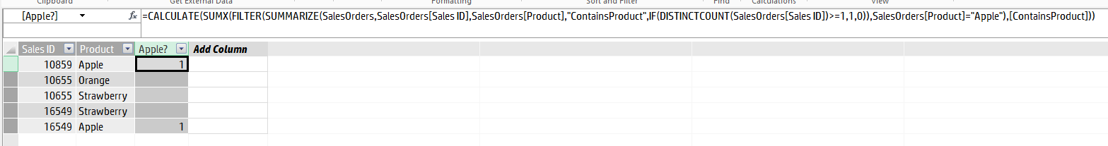
I have a table with sales of individual products, along with their sales order ID. I want to add a calculated column that will indicate if a certain product was contained in the sale. It might be easier to give an example. In this example I want a calculated column that will indicate if the sale included an apple.

Sales ID	Product	Calculated Column Desired Output
10859	Apple	Yes
10655	Orange	No
10655	Strawberry	No
16549	Strawberry	Yes
16549	Apple	Yes

<tbody>
</tbody>

I need a formula that say something like, look for related Sales ID, do any of them contain an Apple, if so Yes, if not No.

Any ideas? Thank you.

 

[svendiamond]

Supposing that table is in columns A, B, and C, and your lookup value "Apple" is in F1, for example, then in C2 and fill down you could use:

=IF(COUNTIFS(A:A,A2,B:B,$F$1)>0,"Yes","No")

That way if apple and that ID show up then you'll get a Yes.

 

[eliwaite]

Thanks svendiamond. That work great in Excel, however I am looking for a solution for PowerPivot. My hangup, is I do not know how to specify a cell reference, like you have down with A2, not sure if it is even possible. Hoping someone here might have a trick up their sleeve.

 

[PowerDAX]

Hi eliwaite....here would be a solution to the calculated column (named the table SalesOrders):

=
CALCULATE (
SUMX (
FILTER (
SUMMARIZE (
SalesOrders,
SalesOrders[Sales ID],
SalesOrders[Product],
"ContainsProduct", IF ( DISTINCTCOUNT ( SalesOrders[Sales ID] ) >= 1, 1, 0 )
),
SalesOrders[Product] = "Apple"
),
[ContainsProduct]
)
)


I would take it one step further and add a calculated field that would work based on filter/slicer selection:

ContainsProduct :=
SUMX (
SUMMARIZE (
SalesOrders,
SalesOrders[Sales ID],
SalesOrders[Product],
"ContainsProduct", IF ( DISTINCTCOUNT ( SalesOrders[Sales ID] ) >= 1, 1, 0 )
),
[ContainsProduct]
)


powerdax.com

 

[eliwaite]

Hi PowerDax. Thank you for your suggestions, I have learned some new tricks from your formulas, however did not quite get the result I was hoping for. Here is a screenshot of the outcome when I utilize your formula:

For Sales ID 16549, I would have expected a "1" for both Strawberry and Apple, however, as you can see that is not the case. Any ideas on how to modify the formula so that Strawberry, for Sales ID 16549 gets a "1" as well?

Thanks,
Eli

 

[scottsen]

I would create a measure, cuz it's fun.
Apple Count := CALCULATE(COUNTROWS(Sales), Sales[Product] = "Apple")

Then use that measure in your calculated column:
Order has Apples := CALCULATE([Apple Count], ALL(Sales), Sales[Sales ID] = EARLIER(Sales[Sales ID])) > 0

 

[PowerDAX]

Sorry...you specified Apple. You would need to state what all of the use cases are where you would expect a one.

If you simply added an OR (or ||) reference as below, it would pick up Strawberry as well. The function I provided will calculate to a "2" for 16549 due to it having both Apple and Strawberry.

SalesOrders[Product] = "Apple" || SalesOrders[Product] = "Strawberry"

or

OR( SalesOrders[Product] = "Apple", SalesOrders[Product] = "Strawberry")

 

[eliwaite]

Hi Scottsen,

Thank you so much, your formulas did the trick.

Not to push my luck but but I want to see if I can eliminate another helper calculated column. I have another table within this PowerPivot model, that contains multiple "indicator" products. Like the Apple in my example, any order that contains an "indicator product, needs to be flagged, as in your case True or False.

My current helper calculated column has the following formula: =IF(SUMX('Product Roster',FIND(UPPER('Product Roster'[Product SKU]),UPPER(SalesOrders[Sku No]),,0))>0,1,0)

In my real spreadsheet anything that results in 1 is my Apple. The reason I am using UPPER is because there are variations on my product SKUs. For example there is APPLE (a new product) and APPLER (a refurbished product) along with some other combinations. The SKU list in the Product Roster only has the SKUs for new products, thus I am looking for anything that contains APPLE.

Any ideas on how to build this directly into the formulas you shared?

Thank you,
Eli

 

[eliwaite]

Hi PowerDAX

I am trying to tag any order that contains a certain product, in this case an Apple regardless of what it is matched up with. This is my desired outcome:

Sales ID	Product	Calculated Column Desired Output
10859	Apple	Yes
10655	Orange	No
10655	Strawberry	No
16549	Strawberry	Yes
16549	Apple	Yes

<tbody>
</tbody>

As you can see order 10655 has an outcome of "No" (or in your formula it would a zero), because that order does not contain an Apple. However order 16549 does contain an Apple, thus all other 16549 Sales ID should be marked with Yes.

 

[Matt Allington]

Why do you want this as a calc column? Presumably you are going to use it for some "next step". What is that next step?