Create Dashboard from data

nparsons75

Well-known Member
Joined
Sep 23, 2013
Messages
1,254
Office Version
  1. 2016
Hi,

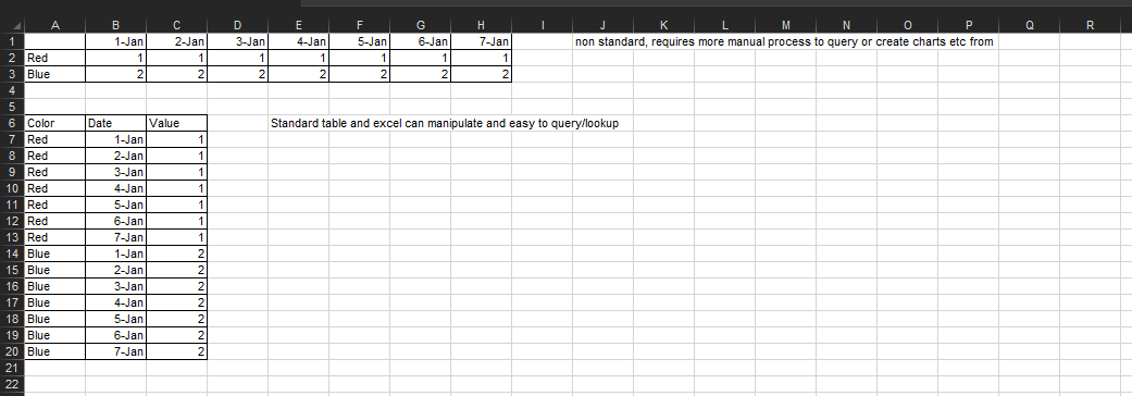
I have a range of data laid out like this. B16:AH21

Dates in the headers of the columns
Data in the rows below the dates.

On my dashboard page I would like to select two criteria.

First, a value from first column.
Second, a date from the column headers.

For example,
In column B I have 5 rows, each row contains a vehicle colour.

RED
GREEN
SILVER
BLACK
WHITE

Across the columns under each date from 1 to 31 depending on the month, there is data. Basically telling me how many of each colour car was sold on that day.

So, from the criteria I choose, I would like to choose colour and data. This will then show all my data in relation to this.
 

Excel Facts

Why does 9 mean SUM in SUBTOTAL?
It is because Sum is the 9th alphabetically in Average, Count, CountA, Max, Min, Product, StDev.S, StDev.P, Sum, VAR.S, VAR.P.
Sheet4

BCDEFGHI
5 Date04/01/2018
6Red3
7Green5
8Silver3
9Black5
10White2
11
12
13
14
15
16 01/01/201802/01/201803/01/201804/01/201805/01/201806/01/201807/01/2018
17Red3133434
18Green4415112
19Silver3513112
20Black4535354
21White5432511

<colgroup><col style="width: 30px; font-weight: bold;"><col style="width: 64px;"><col style="width: 75px;"><col style="width: 75px;"><col style="width: 75px;"><col style="width: 75px;"><col style="width: 75px;"><col style="width: 75px;"><col style="width: 75px;"></colgroup><tbody>
</tbody>

Spreadsheet Formulas
CellFormula
C6=INDEX($C$17:$AG$21,MATCH(B6,$B$17:$B$21,0),MATCH($D$5,$C$16:$AG$16,0))
C7=INDEX($C$17:$AG$21,MATCH(B7,$B$17:$B$21,0),MATCH($D$5,$C$16:$AG$16,0))
C8=INDEX($C$17:$AG$21,MATCH(B8,$B$17:$B$21,0),MATCH($D$5,$C$16:$AG$16,0))
C9=INDEX($C$17:$AG$21,MATCH(B9,$B$17:$B$21,0),MATCH($D$5,$C$16:$AG$16,0))
C10=INDEX($C$17:$AG$21,MATCH(B10,$B$17:$B$21,0),MATCH($D$5,$C$16:$AG$16,0))

<tbody>
</tbody>

<tbody>
</tbody>
 
Upvote 0
Not sure your question but I can tell you that your table is formatted in a non standard way.

Instead of dates going across, the date itself should be part of the data.

Your table heades should be... Color, Date, Value

3 columns with all the data populated...

tQXPeg0.png


I would get into the habit of setting up your tables this way
 
Upvote 0
Thank you, Dryver14 that works perfectly.

For the data I have sheet tabs, 1 for each month of the year. When I change D5, would it be possible for the search to spread across all sheet tabs. For example, If I search for the 14/03/18, could it be that the data is brought in from sheet (MARCH). If I change to 14/04/18 then the data would come from Sheet APRIL. Im not even sure how to explain it properly.....

Fingers crossed. I dont want a dashboard for each month, just one dashboard that can bring rhe data in from any of the sheets that match the date.
 
Upvote 0
If all your tables are laid out the same then you could set a master table lets call it sheets master

Table identical to all the others.

in the cell next to the corner ie next to 01/01/18 and RED type = Sum(.............then select sheet Jan hold shift key and press dec then click on the same cell and press enter

This will give you a sum of all the sheets in that cell then copy down and across. then refer to that table with the index and match
 
Upvote 0
I am not very good with sheet references for formulas so if anyone could help here with formulas for individual sheets or Master sheet that would be good.

I would jump to VBA at this point

(Really must learn indirect function)
 
Upvote 0
Im trying what you suggest but struggling. VBA sounds good, have you got the magic code? ha ha
 
Upvote 0
TBH, I could come up with something but lets see if someone can come up with the indirect formula.

I am studying it as we communicate.

The reason for this is Dashboards work really well if they are mainly formula based, but as long as results are in the same place on each sheet it would not be hard to create a button for each month and show that info when pressed
 
Upvote 0
I guess that wold be the best way. Ive had issues with VBA.... Thanks for all your help, I really appreciate it.
 
Upvote 0
OK, this gives you something to work on. I would suggest naming all the sheets Jan to Dec
Then where I have Sheet5 use a drop down with the months and possibly even Master for the annual figures.

This should give you a good start, anything more just get back in touch and we will work through it


Sheet4

BCDEFGHI
4
5 Date04/01/2018Sheet5
6Red3
7Green5
8Silver3
9Black5
10White2
11
12
13
14
15
16 01/01/201802/01/201803/01/201804/01/201805/01/201806/01/201807/01/2018
17Red3133434
18Green4415112
19Silver3513112
20Black4535354
21White5432511
22
23

<colgroup><col style="width: 30px; font-weight: bold;"><col style="width: 64px;"><col style="width: 75px;"><col style="width: 75px;"><col style="width: 75px;"><col style="width: 75px;"><col style="width: 75px;"><col style="width: 75px;"><col style="width: 75px;"></colgroup><tbody>
</tbody>

Spreadsheet Formulas
CellFormula
C6=INDEX(INDIRECT($E$5&"!$C$17:$AG$21"),MATCH(B6,INDIRECT($E$5&"!$B17:$B21"),0),MATCH($D$5,INDIRECT($E$5&"!$C$16:$AG$16"),0))
C7=INDEX(INDIRECT($E$5&"!$C$17:$AG$21"),MATCH(B7,INDIRECT($E$5&"!$B17:$B21"),0),MATCH($D$5,INDIRECT($E$5&"!$C$16:$AG$16"),0))
C8=INDEX(INDIRECT($E$5&"!$C$17:$AG$21"),MATCH(B8,INDIRECT($E$5&"!$B17:$B21"),0),MATCH($D$5,INDIRECT($E$5&"!$C$16:$AG$16"),0))
C9=INDEX(INDIRECT($E$5&"!$C$17:$AG$21"),MATCH(B9,INDIRECT($E$5&"!$B17:$B21"),0),MATCH($D$5,INDIRECT($E$5&"!$C$16:$AG$16"),0))
C10=INDEX(INDIRECT($E$5&"!$C$17:$AG$21"),MATCH(B10,INDIRECT($E$5&"!$B17:$B21"),0),MATCH($D$5,INDIRECT($E$5&"!$C$16:$AG$16"),0))

<tbody>
</tbody>

<tbody>
</tbody>


Excel tables to the web >> Excel Jeanie
 
Upvote 0

Forum statistics

Threads
1,214,825
Messages
6,121,787
Members
449,049
Latest member
greyangel23

We've detected that you are using an adblocker.

We have a great community of people providing Excel help here, but the hosting costs are enormous. You can help keep this site running by allowing ads on MrExcel.com.
Allow Ads at MrExcel

Which adblocker are you using?

Disable AdBlock

Follow these easy steps to disable AdBlock

1)Click on the icon in the browser’s toolbar.
2)Click on the icon in the browser’s toolbar.
2)Click on the "Pause on this site" option.
Go back

Disable AdBlock Plus

Follow these easy steps to disable AdBlock Plus

1)Click on the icon in the browser’s toolbar.
2)Click on the toggle to disable it for "mrexcel.com".
Go back

Disable uBlock Origin

Follow these easy steps to disable uBlock Origin

1)Click on the icon in the browser’s toolbar.
2)Click on the "Power" button.
3)Click on the "Refresh" button.
Go back

Disable uBlock

Follow these easy steps to disable uBlock

1)Click on the icon in the browser’s toolbar.
2)Click on the "Power" button.
3)Click on the "Refresh" button.
Go back
Back
Top