
New Tips for Excel
October 06, 2006
Recently, I have been out doing several Excel Power Seminars. When you get 150 accountants in a room for a laugh-filled morning of Excel tips and tricks, I always learn something new. Someone in the audience is able to share a cool trick with the rest of the room.
In today's episode, I have a collection of new tricks. These are actually tricks that are better or different than the equivalent method discussed in the book. They will definitely be in the next revision of the book.
By the way, I would love to come to your city to do a Power Excel Seminar. If you belong to a professional group such as the local chapter of the Institute of Managerial Accountants, the Institute of Internal Auditors, the AICPA, the SME, etc., why not suggest that they book me for one of their upcoming CPE days? Send your chapter program chairperson to this page for details.
Find the Difference Between Two Dates
I usually talk about the methods for using =YEAR(), =MONTH(), =DAY() functions, but there is a cool old function hiding in Excel.
The DATEDIF function is left over from Lotus. While Excel help doesn't talk about this function, it is a great way to find the difference between two dates.
The syntax is =DATEDIF(EarlierDate,LaterDate,Code)
Here are the valid values that you can use for Code.
- Y - will tell you the number of complete years between the two dates.
- YM - will tell you the number of complete months, excluding the years, between the two dates.
- MD - will tell you the number of complete days, excluding complete months, between the two dates.
- M - will tell you the number of complete months. For example, I've been alive for 495 months
- D - will tell you the number of days. For example, I've been alive for 15,115 days. This is a trivial use, since you could just subtract one date from another and format as a number to duplicate this code.
The useful codes are the first three codes. On the show, I demonstrated this worksheet. Identical formulas in columns D, E, and F calculate the DATEDIF in years, months, and days.
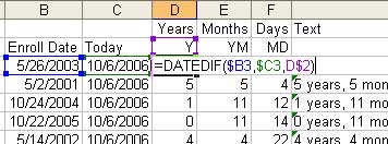
The formula in column G strings this together to create text with the length of time in years, months, and days.
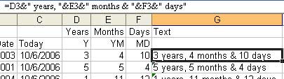
You could combine this into a single formula. If cell A2 contains the joining date, use the following formula in B2:
=DATEDIF($A2,TODAY(),"Y")&" years, "&DATEDIF($A2,TODAY(),"YM")&" months & "&DATEDIF($A2,TODAY(),"MD")&" days"
Sum of Visible Cells
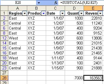
Add a SUM function below a database and then use AutoFilter to filter the database. Excel will annoyingly include the hidden rows in the sum!
Instead, follow these steps:
- Use Data - Filter - AutoFilter to add the AutoFilter dropdowns.
- Choose a Filter for one field
- Go to the blank cell below one of the numeric columns in the database.
- Click the Greek letter E (Sigma) in the standard toolbar. Instead of entering
=SUM(), Excel will enter=SUBTOTAL()and use the codes to prevent hidden rows from being included.
Shortcut key to Repeat the Last Command
The F4 key will repeat the last command that you performed.
For example, select a cell and click the B icon to make the cell bold.
Now, select another cell and press F4. Excel will make that cell bold.
F4 will remember the last command. So, you could make a cell in italics, and then use F4 to make many cells italics.
Pre-select the range of cells to be entered
In the book, I show you how to use Tools - Options - Edit - Move Selection After Enter Direction - Right to force Excel to move to the right when you press the enter key. This is good when you have to enter data going across a row.
It is particularly useful if you are entering numbers on the numeric keypad. The trick allows you to type 123 Enter and end up in the next cell. By keeping your hands on the numeric keypad, you can enter the numbers faster.
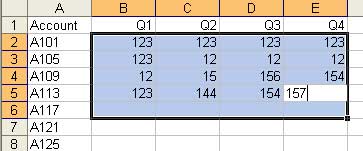
Someone suggested an improvement to this technique. Pre-select the range where you will be entering the data. The advantage is that when you get to the last column and press Enter, Excel will jump to the beginning of the next row.
In the image below, pressing Enter will move you to cell B6.
Ctrl+Drag the Fill Handle
I've shown the Fill Handle trick many times on the show. Enter Monday in A1. If you select cell A1, there is a square dot in the lower right corner of the cell. This dot is the Fill Handle. Click the fill handle and drag either down or to the right. Excel will fill in Tuesday, Wednesday, Thursday, Friday, Saturday, Sunday. If you drag for more than 7 cells, Excel will start over again on Monday.
Excel is really good. It can extend all of these series automatically:
- Monday - Tuesday, Wednesday, Thursday, Friday, etc.
- Jan - Feb, Mar, Apr, etc.
- January - February, March, etc.
- Q1 - Q2, Q3, Q4 etc.
- Qtr 1 - Qtr 2, Qtr 3, Qtr 4, Qtr 1, etc.
- 1st period - 2nd period, 3rd period, 4th period, etc.
- Oct 23 2006 - Oct 24 2006, Oct 25 2006, etc.
Since Excel can do ALL of these amazing series, what would you expect if you enter 1 and drag the fill handle?
You might expect you would get 1, 2, 3, ...
But you really get 1, 1, 1, 1, 1, ...
The book talks about a convoluted method. Enter 1 in A1. Enter 2 in A2. Select A1:A2. Drag the fill handle. There is a better way.
Simply enter 1 in A1. Ctrl+Drag the fill handle. Excel will fill in 1, 2, 3. Holding down the Ctrl seems to override the normal behavior of the fill handle.
Someone in a seminar said that they would like to enter a date, drag the date, and have Excel keep the date the same. If you hold down Ctrl while dragging the fill handle, Excel will override the normal behavior (incrementing the date) and give you the same date in all cells.