
Track Progress Towards a Goal
December 23, 2005
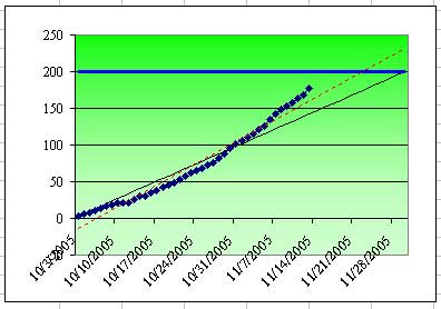
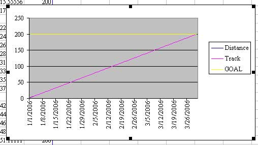
With the new year coming up, you might want to track progress towards some sort of a goal. This cool chart in Excel contains elements that indicate if you are on track to meet a goal. Say that you want to run 250 miles this quarter.
- The black line is the goal
- The blue line is the "on track" line - you have to run 2.7 miles per day to meet the goal
- The green line is the actual miles run
- The red line is the prediction of where you will finish the quarter, based on your progress so far. The red line is by far the coolest part of the chart.
Here is how to create the chart.
-
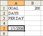
Enter these headings at the top of a worksheet. In cell A5, enter the first date for the chart.
-
Put the cellpointer in A5. You will notice that there is a square dot in the lower right corner of A5. This is the fill handle. With the mouse, grab the fill handle and drag downwards. Watch the tooltip until you see that you've dragged far enough to include the last date of the quarter.

-
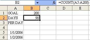
The formula for B2 is
=COUNT(A5:A200). This will count the number of days in your range.
-
The formula for B3 is
=B1/B2. This calculates how far you have to run each day to meet the goal.
-
Use column B to enter how far that you ran each day.

- Although column B contains your actual data, it is not suitable for creating the chart. You will actually build a completely new chart range in columns C:F that will contain the elements needed for the chart.
-
Column C will contain dates. If one axis of your chart range contains numbers or dates, you must leave the top left cell of the chart range blank.
This is a strange bug in Excel - leaving that cell blank will allows Excel's Intellisense to recognize the chart range later. So, leave cell C5 blank, and enter headings for Distance, Track, and Goal in D5:F5.

-
The formula in C5 is
=A5.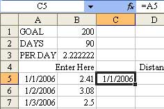
-
Select cell C5. From the menu, select Format Cells. On the Numeric tab, choose the Date category and then the 3/14 format.

- Select cell C5. Drag the fill handle down to copy this formula. Drag down as far as you have data in column A.
-
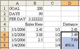
For columns D & E, the formulas in row 5 will be different than those in rows 6 & below. The formulas in row 5 will provide a numeric start. Formulas in row 6 & below will increment those numeric values in row 5. The formula for D5 is
=B5- this will simply copy the first day's distance to the chart range.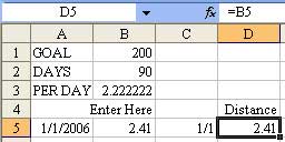
-
In a later step, Excel will add a trendline based on the values in column D. If you merely copied D5 down, you would end up with zeroes for future dates. The zeroes will invalidate the trendline. The trick is that you need to fill future dates with #N/A error values.
In English, then, the formula basically says, "If we ran today, then add today's value to yesterday's total. Otherwise, put an N/A in this cell.
To achieve this result, enter
=IF(NOT(ISBLANK(B6)),D5+B6,NA())in cell D6.
-
Select cell D6. Double click the fill handle to copy this formula down. The double-click trick works because the column to the left of this cell contains values that will guide Excel how far down the formula needs copied.
-
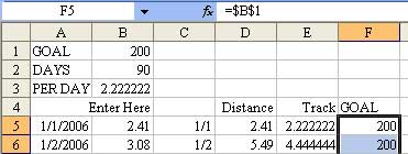
The formula in E5 needs to copy the per day from B3. Enter
=B3in E5. -
The formula for the rest of E needs to add B3 to the previous day. The formula for E6 could be
=E5+B3but this formula would not work when you copy the cell down to the other rows. You always want the formula to add B3 to the cell above.Thus, use
=E5+$B$3in E6. The dollar signs make sure that when you copy the formula, it will always point to B3.
- Move the cellpointer back to E6 and double-click the fill handle to copy the formula down.
-
The formula for all of column F is
=$B$1. This range will be used to draw in the black goal line on the chart. Here is a tip for entering this formula. Start in F5. Type the equals sign. Using the mouse, touch B1. Then, type the F4 key to put the dollar signs in.Hit Ctrl+Enter to accept the formula and stay in the current cell. You can now double-click the fill handle to copy the formula down.
-
Finally, you are ready to create the chart. Select the range of C4:F94. Either use Insert - Chart from the menu, or click the Chart Wizard icon in the standard toolbar.

-
In step 1, choose a Line chart.

-
The chart will require a lot of customization, but none of it happens in the wizard, so just click Finish to create this horrible looking chart.
-
Right-click on the grey background and choose Format Plot Area.

-
Choose Fill Effects.

-
Set up a 2-color gradient as shown here.

-
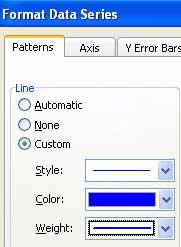
Right-click the yellow Goal series line. Choose Format Data Series.

-
Choose a thick blue line for the goal series.
- Repeat steps 23-24 to change the track line to a thin black line.
-
It is difficult to format the Distance series, as there are only 2 points and it is nearly impossible to see. If it is difficult to right-click an element of the chart, you can use the dropdown in the Charting toolbar.

-
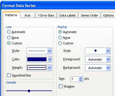
Once the distance series is selected, use the Properties icon to open the Format dialog for the selected series.

-
Add a Marker to this dialog. Change the color to dark blue and the line thickness to medium.
-
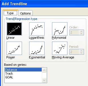
To add the trendline, you will have to be able to right-click on the distance series. This is nearly impossible to do at this point in time. So - I suggest that you "cheat". Enter a fake data point of 20 in cell B7. This will allow you to right-click on the distance series. Choose Add Trendline.

-
On the Trendline dialog, choose the Linear Trendline.
-
Select cell B7 and type the Delete key to erase the fake value there. You will now have the trendline drawn in as a thick black line.

-
Right-click the trend line and choose Format Trendline.
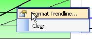
-
Change the Trendline to a broken red line with a thin weight.

-
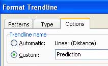
On the Options tab of the Format Trendline, change the series name to Prediction
You now have a completed chart. If you miss a day of running, enter a zero in column B. If you miss a couple of days, the red prediction line will show that you are not on track to make the goal.

You can download the completed chart from this link.