Average/rank with blank cells

[lonewaya1984]

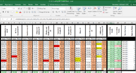
I am an average and self taught excel user so I am not sure if there is a solution to my problem or not. I have built a gradebook for my classes in which I input their percentage grade in one column and in the next it tells me how many points out of the maximum possible for the assignment they earned. (Example assignment worth 20 points if they scored 76% they earned 15.2 points) This is done for each assignment they will do in this block of instruction, 13 in total. At the end of the gradebook I have columns that tell me their GPA average and the next column tells me the total numbers of points they have earned. The next two columns are set to give me their ranking positions in the class one by GPA and the other by total points earned. The problem I am running into is my class can have a maximum of 20 students, but I don't always have 20 students. For example right now I only have 19 in the class. The problem is the rank by GPA breaks and renders the divide by zero error, it does this because the GPA average column as a divide by zero error because the 20th slot has no percentage grades entered under any of the assignments. I tried using the AVERAGEIF formula so the 20th GPA average slot would ignore blank and zero value cells in order to not give the divide by zero error so the ranking function would work but that gives me the "to many arguments error" because I don't have a straight range value, there are two columns with other data between each column that contains the percental grade values. This might have a super easy fix that all my research has eluded me, and it might not be possible at all. This is why I am turning to you all, please help me.

 

[Snakehips]

@lonewaya1984 Welcome

Does something like below help?

Book1
	AP	AQ	AR	AS	AT	AU	AV
5
6		18.09			18
7		22.73			2
8		22.73			2
9		19.45			14
10		19.18			15
11		20.82			10
12		19.73			13
13		20.00			12
14		20.27			11
15
16		18.91			16
17		21.09			9
18		21.36			8
19		21.64			7
20		21.91			6
21		22.18			5
22		22.45			4
23		18.36			17
24		23.00			1
25
SERVERS & OPTIONS

Cell Formulas
Range	Formula
AQ6:AQ25	AQ6	=IFERROR(AVERAGE(D6,G6,J6,M6,P6,S6,V6,Y6,AB6,AE6,AH6,AK6,AN6),"")
AT6:AT25	AT6	=IFERROR(RANK(AQ6,$AQ$6:$AQ$25,0),"")

 

[lonewaya1984]

@lonewaya1984 Welcome

Does something like below help?

Book1
	AP	AQ	AR	AS	AT	AU	AV
5
6		18.09			18
7		22.73			2
8		22.73			2
9		19.45			14
10		19.18			15
11		20.82			10
12		19.73			13
13		20.00			12
14		20.27			11
15
16		18.91			16
17		21.09			9
18		21.36			8
19		21.64			7
20		21.91			6
21		22.18			5
22		22.45			4
23		18.36			17
24		23.00			1
25
SERVERS & OPTIONS

Cell Formulas
Range	Formula
AQ6:AQ25	AQ6	=IFERROR(AVERAGE(D6,G6,J6,M6,P6,S6,V6,Y6,AB6,AE6,AH6,AK6,AN6),"")
AT6:AT25	AT6	=IFERROR(RANK(AQ6,$AQ$6:$AQ$25,0),"")

This absolutely did the trick, your are the BEST!! Thanks so much for your help and speedy reply!!!!!!!