Hello
I am trying to calculate and then chart the difference between dates in a pivot table and I could use some help.
I have a list of dated transactions for various customers and I am trying to find the time elapsed since the previous payment so that I can show it in a stacked column chart. There could be any number of payments for a given customer and multiple payments could be received on the same day. Also each payment is labeled ("#1", "#2", "Deposit", "Prepayment", etc) and I'd like those labels to be reflected in the legend of the chart.
I am trying to do this with pivot tables because I am working with imported Quickbooks data. I want to be able to paste a huge list of transactions from QB that has all the info I need, then simply click refresh on my pivot tables and everything updates. I already have a bunch of other pivot tables and charts I've put together that work like this without me needing to clean/process the data in any way.
I'm sure I need to use Values with Show Values As "Difference From" but I cannot figure out how to get it to work. The values in the table always end up as either N/A, 1, or the date itself. I've tried tons of variations of different Base Fields and Base Items and I can't figure it out.
For example, if Customer A payment #1 received 1/1/21, payment #2 received 1/11/21, then payment #3 received 1/26/21, then there would be a stacked column chart with a column for Customer A and that column would have two segments, one of value 10 (labeled "payment #2") and the next of value 15 (labeled "payment #3").
Does that make sense? Ultimately I'm trying to get a visualization showing: this is how long each customer/project took and this is how long it was between payments for each customer.
Here are some example transactions:
Here is what my pivot table currently looks like:
Fields:

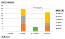
Which creates a stacked column chart that is almost what I want except that the vertical axis should be # of days not raw date.

Any help would be greatly appreciated.
I am trying to calculate and then chart the difference between dates in a pivot table and I could use some help.
I have a list of dated transactions for various customers and I am trying to find the time elapsed since the previous payment so that I can show it in a stacked column chart. There could be any number of payments for a given customer and multiple payments could be received on the same day. Also each payment is labeled ("#1", "#2", "Deposit", "Prepayment", etc) and I'd like those labels to be reflected in the legend of the chart.
I am trying to do this with pivot tables because I am working with imported Quickbooks data. I want to be able to paste a huge list of transactions from QB that has all the info I need, then simply click refresh on my pivot tables and everything updates. I already have a bunch of other pivot tables and charts I've put together that work like this without me needing to clean/process the data in any way.
I'm sure I need to use Values with Show Values As "Difference From" but I cannot figure out how to get it to work. The values in the table always end up as either N/A, 1, or the date itself. I've tried tons of variations of different Base Fields and Base Items and I can't figure it out.
For example, if Customer A payment #1 received 1/1/21, payment #2 received 1/11/21, then payment #3 received 1/26/21, then there would be a stacked column chart with a column for Customer A and that column would have two segments, one of value 10 (labeled "payment #2") and the next of value 15 (labeled "payment #3").
Does that make sense? Ultimately I'm trying to get a visualization showing: this is how long each customer/project took and this is how long it was between payments for each customer.
Here are some example transactions:
| Date | Customer | Memo | Amount |
| 3/9/2021 | Customer C | Draw #5 | 26339 |
| 4/14/2021 | Customer J | Draw #1 | 21447 |
| 4/23/2021 | Customer D | Draw #1 | 10263 |
| 5/18/2021 | Customer H | Draw #5 | 16948 |
| 5/24/2021 | Customer J | Draw #2 | 28596 |
| 6/21/2021 | Customer D | Draw #2 | 13684 |
| 6/21/2021 | Customer J | Draw #3 | 28596 |
| 6/23/2021 | Customer H | Draw #6 | 11299 |
| 8/25/2021 | Customer D | Draw #3 | 13684 |
| 9/9/2021 | Customer J | Draw #4 | 28596 |
| 10/12/2021 | Customer D | Draw #4 | 13684 |
Here is what my pivot table currently looks like:
| income and expenses TEST.xlsx | ||||||||||
|---|---|---|---|---|---|---|---|---|---|---|
| A | B | C | D | E | F | G | H | |||
| 3 | Sum of Date | Column Labels | ||||||||
| 4 | Row Labels | Draw #1 | Draw #2 | Draw #3 | Draw #4 | Draw #5 | Draw #6 | Grand Total | ||
| 5 | Customer A | 10/14/2021 | 11/23/2021 | 1/25/2022 | 2/28/2022 | 4/1/2022 | 4/8/2022 | 6/13/2632 | ||
| 6 | Customer B | 3/3/2022 | 4/14/2022 | 5/19/2022 | 6/22/2022 | 7/25/2022 | 11/21/2511 | |||
| 7 | Customer C | 3/9/2021 | 3/9/2021 | |||||||
| 8 | Customer D | 4/23/2021 | 6/21/2021 | 8/25/2021 | 10/12/2021 | 11/16/2021 | 1/14/2022 | 2/23/2630 | ||
| 9 | Customer E | 10/22/2021 | 11/15/2021 | 2/1/2022 | 3/8/2022 | 5/13/2022 | 5/13/2022 | 9/13/2632 | ||
| 10 | Customer F | 3/21/2022 | 4/14/2022 | 5/24/2022 | 7/1/2022 | 5/29/2389 | ||||
| 11 | Customer G | 12/8/2021 | 3/12/2022 | 3/31/2022 | 5/11/2022 | 7/18/2022 | 7/18/2022 | 11/5/2633 | ||
| 12 | Customer H | 5/18/2021 | 6/23/2021 | 11/10/2142 | ||||||
| 13 | Customer I | 12/28/2021 | 2/4/2022 | 2/28/2022 | 4/20/2022 | 5/22/2022 | 7/1/2022 | 6/16/2633 | ||
| 14 | Customer J | 4/14/2021 | 5/24/2021 | 6/21/2021 | 9/9/2021 | 11/16/2021 | 12/30/2021 | 9/26/2629 | ||
| 15 | Customer K | 7/1/2022 | 7/1/2022 | |||||||
| 16 | Grand Total | 1/13/2997 | 7/10/2875 | 6/26/2876 | 6/22/2877 | 6/17/2998 | 3/19/2755 | 3/19/7880 | ||
Sheet1 | ||||||||||
Fields:
Which creates a stacked column chart that is almost what I want except that the vertical axis should be # of days not raw date.
Any help would be greatly appreciated.