Compare Caliper Measurements

[Andreavnn]

Hello,

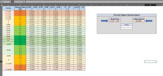
I am looking for help to correct my formula. I am wanting to have a USER input a 'Thread Size' into J7 which references a column [C through G] and then input a 'Caliper Result' which is a decimal value into L7. Using the information is J7 and L7 that formula will select the closest result based on the decimal input in L7 and the column selected J7 and then display the matching results in column B and A, K10 and K11.

 

[DanteAmor]

Hi @Andreavnn , I hope you are well.

Put the following formula in cell K10, for the result in column B:

=INDEX(B1:B32,LARGE(IF(INDEX(C2:G32,,MATCH(J7,C1:G1,0))>=L7,ROW(B2:B32)),1))

Put the following formula in cell K11, for the result in column A:

=INDEX(A1:A32,LARGE(IF(INDEX(C2:G32,,MATCH(J7,C1:G1,0))>=L7,ROW(B2:B32)),1))

I suggest that in column A you fill in all the data, otherwise it will return 0 or empty in the cells where you have no information:

Dante Amor
	A
1	Turns
2	1-1/2T
3	1-1/2T
4	1-1/2T
5	1-1/4T
6	1-1/4T
7	1
8	1
9	3/4T
10	3/4T
11	3/4T
12	1/2T
13	1/2T
14	1/2T
Hoja7

--------------
Let me know the result and I'll get back to you as soon as I can.
Cordially
Dante Amor
--------------​

 

[DanteAmor]

Or this:

Put the following formula in cell K10, for the result in column B:

=INDEX(A2:B32,MATCHX(L7,FILTER(C2:G32,C1:G1=J7),1),2)

Put the following formula in cell K11, for the result in column A:

=INDEX(A2:B32,MATCHX(L7,FILTER(C2:G32,C1:G1=J7),1),1)

 

[Andreavnn]

This work, but for some reason it seems to be off a few cells when inputting data into L7.

K10

=IFERROR(INDEX(B3:B33,LARGE(IF(INDEX(C3:G33,,MATCH(J8,C1:G1,0))>=L8,ROW(B3:B33)),1)),"")

K11

=IFERROR(INDEX(A3:A33,LARGE(IF(INDEX(C3:G33,,MATCH(J8,C1:G1,0))>=L8,ROW(B3:B33)),1)),"")

You can see in the image I put in '-0.0519' which should be '-1.4' or '-1-1/4T' I can't seem to get it to function correctly. It will also display blanks sometimes too, you can see in my second image.

I did add the following to the C3-G3:C33-G33 - which will auto-calculate the decimals in those columns to ensure accuracy.

=1/$C$2*$B3

I played with it some, but can't seem to get it to function correctly.

EDIT* Column 'A' does have information in each cell I just changed the text color to match the background color for visual design.

 

[DanteAmor]

It will also display blanks sometimes too, you can see in my second image.

I suggest that in column A you fill in all the data, otherwise it will return 0 or empty in the cells where you have no information:

 

[Andreavnn]

I placed data in column 'A' and the return is still off. Using '1' or '-1' in the [match_type] doesn't seem to fix it either. Maybe I am doing something wrong?

If I changed the LARGE(array, K) from 1 to 3 everything works, but the results from '1.4' to '1.5' in each column. Both K10 & K11 return blanks.

 

[DanteAmor]

In your user profile data it says you have office 365.
You shouldn't have any problems with the formulas:

If not, in the case of this formula you must enter it with an array formula:

varios 12jun2023.xlsm
	A	B	C	D	E	F	G	H	I	J	K	L
1	Turns		1/6" -1/8"	1/4" - 3/8"	1/2" - 3/4"	1" - 2"	2 1/2" - 4"
2	1-1/2T	1-5	0.0556	0.0833	0.1071	0.1304	0.1875
3	1-1/2T	1-4	0.0519	0.0796	0.1034	0.1267	0.1838
4	1-1/2T	1-3	0.0482	0.0759	0.0997	0.1230	0.1801
5	1-1/4T	1-2	0.0445	0.0722	0.0960	0.1193	0.1764
6	1-1/4T	1-1	0.0408	0.0685	0.0923	0.1156	0.1727			Thread Size		Caliper Result
7	1	1	0.0371	0.0648	0.0886	0.1119	0.1690			1/6" -1/8"		0.0556
8	1	0.9	0.0334	0.0611	0.0849	0.1082	0.1653
9	3/4T	0.8	0.0297	0.0574	0.0812	0.1045	0.1616				Turns
10	3/4T	0.7	0.0260	0.0537	0.0775	0.1008	0.1579				1-5	B
11	3/4T	0.6	0.0223	0.0500	0.0738	0.0971	0.1542				1-1/2T	A
12	1/2T	0.5	0.0186	0.0463	0.0701	0.0934	0.1505
13	1/2T	0.4	0.0149	0.0426	0.0664	0.0897	0.1468
14	1/2T	0.3	0.0112	0.0389	0.0627	0.0860	0.1431
Hoja7

Cell Formulas
Range	Formula
K10	K10	=INDEX(B1:B14,LARGE(IF(INDEX(C2:G14,,MATCH(J7,C1:G1,0))>=L7,ROW(B2:B14)),1))
K11	K11	=INDEX(A1:A14,LARGE(IF(INDEX(C2:G14,,MATCH(J7,C1:G1,0))>=L7,ROW(B2:B14)),1))
Press CTRL+SHIFT+ENTER to enter array formulas.

Note:
Check that the data you type in cell J7 exactly matches any data in cells C1 through G1.