Conditional Formatting IF AND

[CordingBags]

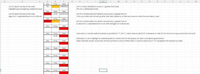
Have a spreadsheet with times in one column and dates in another.
Trying to remind the user that if there is a date in one column then there must be a time in the other.

Have used both =NOT(ISBLANK(F2)) and =(ISBLANK(F2)) both of which provide a bit of a messy workaround

Ideally I would have a conditional formatting rule formula that clears the fill colour if the itself is populated.

ie IF CELL F2 has a date, CELL E2 highlights until it also has a time.

Logic IF cell F2 has a date AND this cell (E2) is blank then highlight E2.

Notes: Both columns are blank at the beginning of the process, both columns are DATA Validation controlled to ensure only a date in one and time in the other is accepted.

The more difficult challenge is to reverse the process in column F where the dates already have a conditional formatting rule to ensure that each one is greater than the entry above.
So I very much suspect that whilst a clever formula may allow for the IF AND logic it will not also accommodate the is greater than previous.
However a missing date against a time is less important.


Appreciate any help

Thanks

Paul

 

[etaf]

this should work for a blank time , where there is a date entry
=AND($F2<>"", $E2="" )

for 2007, 2010 , 2013 , 2016 , 2019 or 365 Subscription excel version
Conditional Formatting

Highlight applicable range >>
E2:E100 - Change, reduce or extend the rows to meet your data range of rows

Home Tab >> Styles >> Conditional Formatting
New Rule >> Use a formula to determine which cells to format
Edit the Rule Description: Format values where this formula is true:
=AND($F2<>"", $E2="" )

Format [Number, Font, Border, Fill]
choose the format you would like to apply when the condition is true
OK >> OK

how does the greater than previous date work - does that also use the time , i assume you would get the same date entry a few times ??

maybe we need an example
Therefore -

A SMALL sample spreadsheet, around 10-20 rows, would help a lot here, with all sensitive data removed, and expected results mocked up and manually entered, with a few notes of explanation.

This will possibly enable a quicker and more accurate solution for you.

MrExcel has a tool called “XL2BB” that lets you post samples of your data and will allow us to copy/paste your sample data into our Excel spreadsheets, saving a lot of time.

XL2BB - Excel Range to BBCode

Excel 'mini-sheet' in messages - XL2BB Although experts prefer to read your description and question instead of working in your actual file to solve your problem, there are times that it is difficult to explain an issue without providing actual...

www.mrexcel.com

You can also test to see if it works ok, in the "Test Here" forum.

Test Here

Use this forum to test your signature, learn bbcode, smilies, XL2BB, etc. Threads in this forum are automatically deleted after no replies for seven (7) days

www.mrexcel.com

OR if you cannot get XL2BB to work, or have restrictions on your PC

then put the sample spreadsheet onto a share

I only tend to goto OneDrive, Dropbox or google docs , as I'm never certain of other random share sites and possible virus.
Please make sure you have a representative data sample and also that the data has been desensitised, remember this site is open to anyone with internet access to see - so any sensitive / personal data should be removed

Make sure you set any share or google to share to everyone

 

[CordingBags]

this should work for a blank time , where there is a date entry
=AND($F2<>"", $E2="" )

for 2007, 2010 , 2013 , 2016 , 2019 or 365 Subscription excel version
Conditional Formatting

Highlight applicable range >>
E2:E100 - Change, reduce or extend the rows to meet your data range of rows

Home Tab >> Styles >> Conditional Formatting
New Rule >> Use a formula to determine which cells to format
Edit the Rule Description: Format values where this formula is true:
=AND($F2<>"", $E2="" )

Format [Number, Font, Border, Fill]
choose the format you would like to apply when the condition is true
OK >> OK

how does the greater than previous date work - does that also use the time , i assume you would get the same date entry a few times ??

maybe we need an example
Therefore -

A SMALL sample spreadsheet, around 10-20 rows, would help a lot here, with all sensitive data removed, and expected results mocked up and manually entered, with a few notes of explanation.

This will possibly enable a quicker and more accurate solution for you.

MrExcel has a tool called “XL2BB” that lets you post samples of your data and will allow us to copy/paste your sample data into our Excel spreadsheets, saving a lot of time.

XL2BB - Excel Range to BBCode

Excel 'mini-sheet' in messages - XL2BB Although experts prefer to read your description and question instead of working in your actual file to solve your problem, there are times that it is difficult to explain an issue without providing actual...

www.mrexcel.com

You can also test to see if it works ok, in the "Test Here" forum.

Test Here

Use this forum to test your signature, learn bbcode, smilies, XL2BB, etc. Threads in this forum are automatically deleted after no replies for seven (7) days

www.mrexcel.com

OR if you cannot get XL2BB to work, or have restrictions on your PC

then put the sample spreadsheet onto a share

I only tend to goto OneDrive, Dropbox or google docs , as I'm never certain of other random share sites and possible virus.
Please make sure you have a representative data sample and also that the data has been desensitised, remember this site is open to anyone with internet access to see - so any sensitive / personal data should be removed

Make sure you set any share or google to share to everyone

The suggested Conditional Formatting for the TIME column worked with a little tweaking, =AND(F5<>"", E5="" ), had to remove the absolute references in order to copy it around the workbook.
I have tried to create an XL2BB but not sure how successful I have been to show the greater challenge in the DATE column.

Is this what XL2bb should look like?

Date and Time checks.xlsm
	A	B	C	D	E	F	G	H	I	J	K	L	M	N	O	P	Q	R	S	T	U	V	W
1				Day	Time	Date
2		Cell D2 reports the day of the week		Thu		14/09/2023		Cell F2 is Data Validated to ensure it is greater than today
3		Highlighting but accepting a weekend fixture						This row is deliberately blank
4				Day	Time	Date
5		Cell D5 reports the day of the week		Sat	14:30	16/09/2023		Cell F5 is Conditionally Formatted to ensure entry is greater than F2
6		Again this is replicated down to row 300+ etc.						I only use conditional formatting rather than Data Validation as there are occasions when the same date is used
7				Day	Time	Date
8				Sun		17/09/2023		Cell F8 is Conditionally Formatted to ensure entry is greater than F5
9								As above this is replicated down to row 300+ and again on multiple tabs
10				Day	Time	Date
11
12
13				Day	Time	Date		Time column is conditionally formatted using =AND(F5<>"", E5="" ), had to remove ABSOLUTE $ reference in order for this formula to copy around the work book
14					18:30
15								Date column is all in highlight at commencement as Conditional Formatting does not seem to be able to ignore blanks.
16				Day	Time	Date		Ideally the Date column would start unfilled, but then to colour if either there is a time in column E or if it is not greater than the previous date.
17
18
19				Day	Time	Date
20
21
22				Day	Time	Date
23
24
25				Day	Time	Date
26
27
28				Day	Time	Date
29
30
31				Day	Time	Date
Sheet1

Cell Formulas
Range	Formula
D2,D29,D26,D23,D20,D17,D14,D11,D8,D5	D2	=IF(F2<1,"",WEEKDAY(F2))

Cells with Conditional Formatting
Cell	Condition		Cell Format	Stop If True
E29	Expression	=AND(F29<>"", E29="" )	text	YES
E26	Expression	=AND(F26<>"", E26="" )	text	YES
E23	Expression	=AND(F23<>"", E23="" )	text	YES
E30	Expression	=NOT(ISBLANK(E30))	text	YES
E27	Expression	=NOT(ISBLANK(E27))	text	YES
E24	Expression	=NOT(ISBLANK(E24))	text	YES
E20	Expression	=AND(F20<>"", E20="" )	text	YES
E17	Expression	=AND(F17<>"", E17="" )	text	YES
E14	Expression	=AND(F14<>"", E14="" )	text	YES
E11	Expression	=AND(F11<>"", E11="" )	text	YES
E8	Expression	=AND(F8<>"", E8="" )	text	YES
E5	Expression	=AND(F5<>"", E5="" )	text	YES
E2	Expression	=AND(F2<>"", E2="" )	text	YES
D29	Cell Value	=1	text	YES
D29	Cell Value	=7	text	YES
D26	Cell Value	=1	text	YES
D26	Cell Value	=7	text	YES
D23	Cell Value	=1	text	YES
D23	Cell Value	=7	text	YES
D20	Cell Value	=1	text	YES
D20	Cell Value	=7	text	YES
D17	Cell Value	=1	text	YES
D17	Cell Value	=7	text	YES
D14	Cell Value	=1	text	YES
D14	Cell Value	=7	text	YES
D11	Cell Value	=1	text	YES
D11	Cell Value	=7	text	YES
D8	Cell Value	=1	text	YES
D8	Cell Value	=7	text	YES
D5	Cell Value	=1	text	YES
D5	Cell Value	=7	text	YES
E21	Expression	=NOT(ISBLANK(E21))	text	YES
F30	Expression	=NOT(ISBLANK(F30))	text	YES
D30	Expression	=NOT(ISBLANK(D30))	text	YES
F27	Expression	=NOT(ISBLANK(F27))	text	YES
D27	Expression	=NOT(ISBLANK(D27))	text	YES
F24	Expression	=NOT(ISBLANK(F24))	text	YES
D24	Expression	=NOT(ISBLANK(D24))	text	YES
F21	Expression	=NOT(ISBLANK(F21))	text	YES
E21	Expression	=NOT(ISBLANK(E21))	text	YES
D21	Expression	=NOT(ISBLANK(D21))	text	YES
F18	Expression	=NOT(ISBLANK(F18))	text	YES
E18	Expression	=NOT(ISBLANK(E18))	text	YES
D18	Expression	=NOT(ISBLANK(D18))	text	YES
F15	Expression	=NOT(ISBLANK(F15))	text	YES
E15	Expression	=NOT(ISBLANK(E15))	text	YES
D15	Expression	=NOT(ISBLANK(D15))	text	YES
F12	Expression	=NOT(ISBLANK(F12))	text	YES
E12	Expression	=NOT(ISBLANK(E12))	text	YES
D12	Expression	=NOT(ISBLANK(D12))	text	YES
F9	Expression	=NOT(ISBLANK(F9))	text	YES
E9	Expression	=NOT(ISBLANK(E9))	text	YES
D9	Expression	=NOT(ISBLANK(D9))	text	YES
F6	Expression	=NOT(ISBLANK(F6))	text	YES
E6	Expression	=NOT(ISBLANK(E6))	text	YES
D6	Expression	=NOT(ISBLANK(D6))	text	YES
F3	Expression	=NOT(ISBLANK(F3))	text	YES
E3	Expression	=NOT(ISBLANK(E3))	text	YES
D3	Expression	=NOT(ISBLANK(D3))	text	YES
F29	Cell Value	<=F26	text	YES
F26	Cell Value	<=F23	text	YES
F23	Cell Value	<=F20	text	YES
F20	Cell Value	<=F17	text	YES
F17	Cell Value	<=F14	text	YES
F14	Cell Value	<=F11	text	YES
F11	Cell Value	<=F8	text	YES
F8	Cell Value	<=F5	text	YES
F5	Cell Value	<=F2	text	YES
D2	Cell Value	=1	text	YES
D2	Cell Value	=7	text	YES
F2	Cell Value	<TODAY()	text	YES

Cells with Data Validation
Cell	Allow	Criteria
D8	List	=$A$1
D11	List	=$A$1
D14	List	=$A$1
D17	List	=$A$1
D23	List	=$A$1
D29	List	=$A$1
F19:F20	Date	between 01/01/2023 and 31/12/2100
F25:F26	Date	between 01/01/2023 and 31/12/2100
D5	List	=$A$1
E5	Time	between 00:01:00 and 23:59:00
F5	Date	between 01/01/2023 and 31/12/2100
D20	List	=$A$1
E20	Time	between 00:01:00 and 23:59:00
D26	List	=$A$1
E26	Time	between 00:01:00 and 23:59:00
E1	Time	between 00:01:00 and 23:59:00
E7	Time	between 00:01:00 and 23:59:00
F7:F8	Date	between 01/01/2023 and 31/12/2100
E8	Time	between 00:01:00 and 23:59:00
E16	Time	between 00:01:00 and 23:59:00
F16:F17	Date	between 01/01/2023 and 31/12/2100
E17	Time	between 00:01:00 and 23:59:00
E10	Time	between 00:01:00 and 23:59:00
F10:F11	Date	between 01/01/2023 and 31/12/2100
E11	Time	between 00:01:00 and 23:59:00
E13	Time	between 00:01:00 and 23:59:00
F13:F14	Date	between 01/01/2023 and 31/12/2100
E14	Time	between 00:01:00 and 23:59:00
E22	Time	between 00:01:00 and 23:59:00
F22:F23	Date	between 01/01/2023 and 31/12/2100
E23	Time	between 00:01:00 and 23:59:00
E28	Time	between 00:01:00 and 23:59:00
F28:F29	Date	between 01/01/2023 and 31/12/2100
E29	Time	between 00:01:00 and 23:59:00
E31	Time	between 00:01:00 and 23:59:00
F31:F32	Date	between 01/01/2023 and 31/12/2100
D2	List	=$A$1
E2	Time	between 00:01:00 and 23:59:00
F2	Date	>TODAY()

.

Much appreciate the help
Thanks
Paul

 

[etaf]

a blank is seen as a date as dates are just number so to stop that just add an
AND( cell <> "", rest of rule.......

a similar formula for testing if a date is blank and time entered

=AND(E5<>"", F5="" )
Not sure why you choose F5 , when data starts at F2
also loads of conditional formatting rules used - you can apply to a range , dont need to add to every cell

then to test for the date

something like

=AND(F2<>"",F2<>"date",F2<MAX($F$2:F2))
and applied to F2toF100

so i only have 1 conditional formatting rule - but have set to ignore cells with DATE in and also blanks

Book6
	A	B	C	D	E	F
1						Date
2						9/14/23
3
4						Date
5						9/16/23
6
7						Date
8						9/17/23
9
10						Date
11						8/16/23
12
13						Date
14
15
16						Date
17
18
19						Date
20
21
22						Date
23
24
25						Date
26
27
28						Date
29
30
31						Date
32
33
34
Sheet2

Cells with Conditional Formatting
Cell	Condition		Cell Format	Stop If True
F2:F100	Expression	=AND(F2<>"",F2<>"date",F2<MAX($F$2:F2))	text	YES

for 2007, 2010 , 2013 , 2016 , 2019 or 365 Subscription excel version
Conditional Formatting

Highlight applicable range >>
F2:F100 - Change, reduce or extend the rows to meet your data range of rows

Home Tab >> Styles >> Conditional Formatting
New Rule >> Use a formula to determine which cells to format
Edit the Rule Description: Format values where this formula is true:
=AND(F2<>"",F2<>"date",F2<MAX($F$2:F2))

Format [Number, Font, Border, Fill]
choose the format you would like to apply when the condition is true
OK >> OK

 

[CordingBags]

a blank is seen as a date as dates are just number so to stop that just add an
AND( cell <> "", rest of rule.......

a similar formula for testing if a date is blank and time entered

=AND(E5<>"", F5="" )
Not sure why you choose F5 , when data starts at F2
also loads of conditional formatting rules used - you can apply to a range , dont need to add to every cell

then to test for the date

something like

=AND(F2<>"",F2<>"date",F2<MAX($F$2:F2))
and applied to F2toF100

so i only have 1 conditional formatting rule - but have set to ignore cells with DATE in and also blanks

Book6
	A	B	C	D	E	F
1						Date
2						9/14/23
3
4						Date
5						9/16/23
6
7						Date
8						9/17/23
9
10						Date
11						8/16/23
12
13						Date
14
15
16						Date
17
18
19						Date
20
21
22						Date
23
24
25						Date
26
27
28						Date
29
30
31						Date
32
33
34
Sheet2

Cells with Conditional Formatting
Cell	Condition		Cell Format	Stop If True
F2:F100	Expression	=AND(F2<>"",F2<>"date",F2<MAX($F$2:F2))	text	YES

for 2007, 2010 , 2013 , 2016 , 2019 or 365 Subscription excel version
Conditional Formatting

Highlight applicable range >>
F2:F100 - Change, reduce or extend the rows to meet your data range of rows

Home Tab >> Styles >> Conditional Formatting
New Rule >> Use a formula to determine which cells to format
Edit the Rule Description: Format values where this formula is true:
=AND(F2<>"",F2<>"date",F2<MAX($F$2:F2))

Format [Number, Font, Border, Fill]
choose the format you would like to apply when the condition is true
OK >> OK

Many Thanks for your help, yes got there.
Cheers
Paul

 

[etaf]

you are welcome