How to use add a criteria to filter my data

[iQuikDraw]

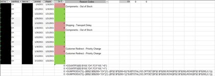
So, in the attached screenshots, I have 2 tables. I am using 2 images here, one each showing the highlight on a "Late" or "On Time" cell so you can see the same formula except I change a "0" to a "!". Now this formula gives me the entire total from the worksheet being queried, not down to the specific warehouse in column B. Every time I try to include that as another criteria in either formula, and get past any syntax errors, either formula only returns "0" when I know there should be a resulting count. I also realize that if I can get a working formula, I wont have to use the "103,OFFSET" part since I don't want to navigate to a bunch of tabs to manually filter each one and have this formula ignoring hidden cells. If it works right, nothing needs be hidden at all manually...At least that's what I'm tying to do

The table on the left is created by a VB script and basically all imported shipping data for a given week (With a worksheet created and named for that week.). On a summary data tab, I have the second table where I want to count the number of rows where the "On Time" column (Column F) shows a 1 for a given warehouse in column B. I want to plug this into my VB script to merely populate the summary data table with the same formula every time a new worksheet gets created for that week for each of the warehouses showing. Instead of charting from VB, I only want to drop a formula in each cell on the summary page, to pull the data from the other page.

To get this working, I have tried "SUMPRRODUCT" formulas mostly, COUNTIFS as well, but I just can't seem to get the formula to include the reference back to the specific warehouse.


=SUMPRODUCT((F2:F200=0)*(SUBTOTAL(103,OFFSET(F2:F200,ROW(F2:F200)-MIN(ROW(F2:F200)),0,1))))

=SUMPRODUCT((F2:F200=1)*(SUBTOTAL(103,OFFSET(F2:F200,ROW(F2:F200)-MIN(ROW(F2:F200)),0,1))))


Is there a way to expand this formula to count only if the warehouse (In column B) is A, B, or C?

If not, is there a different function that will include that and get me the same resulting data for my summary table broken down that specific?

I'm using this table solely to build a running year chart that shows the weekly (Which means pulling data from...all...the weekly tabs as they occur.) "on time/late" bars over the YTD for each specific warehouse.

Can someone help me sort this out?

 

[maabadi]

Try this:

=SUMPRODUCT(--($F$2:$F$200=0)*SUBTOTAL(103,OFFSET($F$2:$F$200,ROW($F$2:$F$200)-ROW($F$2),0,1)))

 

[iQuikDraw]

Try this:

=SUMPRODUCT(--($F$2:$F$200=0)*SUBTOTAL(103,OFFSET($F$2:$F$200,ROW($F$2:$F$200)-ROW($F$2),0,1)))

I tried that. That again returns totals of the whole data table, not sorted out by way of column "B". As an example, this is what I am trying to add:

=SUMPRODUCT(--($B$2:$B$200="CH")*(--($F$2:$F$200=1)*SUBTOTAL(103,OFFSET($F$2:$F$200,ROW($F$2:$F$200)-ROW($F$2),0,1))))

This does not cause any errors but only returns ")" no matter if I change it to "1" or "0" for the "F" column 0 or 1. I am trying to sort the data relative to column "B" which is warehouse specific. Maybe this is the wrong formula to try to do in this context, or, I have the syntax wrong?

 

[maabadi]

What About:

=SUMPRODUCT((--($B$2:$B$200="CH"))*(--($F$2:$F$200=0))*SUBTOTAL(103,OFFSET($F$2:$F$200,ROW($F$2:$F$200)-ROW($F$2),0,1)))

 

[iQuikDraw]

Here is a little simpler approach.

Here I am showing a list where I manually filtered the worksheet to specifically show the warehouse specific rows. For the warehouse "CH" in column B, I want to know how many times (Rows) the shipments were "On Time" or "Late".

At the bottom right corner, I have 4 cells where I first try to use COUNTIFS formulas to sort based on column B combined with column F to tell me number of times they were "1" or "0". Then I tried the same thing with the SUMPRODUCT formulas. The next column over I show the text version of the formulas, all of which return "0" regardless of what the sorted list is showing. In this case, it should be 8 on time and 5 late. or 8 x 1 and 5 x 0...In total there are 62 entries with 12 late shipments, if the entire sheet is not filtered. Formulas should still return the same counts, filtered or not.

I checked the B column to see if where I am asking it to match "CH" has no leading or trailing characters throwing of the "CH" reference due to hidden character spaces, etc. I found none. None of these formulas returned any errors but will not give counts other than 0.

 

[maabadi]

Please upload your example file & Desired Results with XL2BB ADDIN (Preferable) OR upload it at free uploading site e.g. www.dropbox.com or googledrive or onedrive and insert link here.

 

[iQuikDraw]

Well I cut this down to the single worksheet in question. I hope I provided everything needed to sort the formula(s) out.

Example_File_1.xlsm
	A	B	C	D	E	F	G	H	I	J	K	L	M	N	O	P
1	ord no	warehouse	item no	promise dt	shipped dt	On Time
2		AT		1/29/2021	1/19/2021	1
3		AT		2/26/2021	1/19/2021	1
4		CA		3/1/2021	1/19/2021	1
5		CH		1/4/2021	1/19/2021	0
6		AT		1/25/2021	1/19/2021	1
7		CH		1/21/2021	1/19/2021	1
8		AT		1/22/2021	1/19/2021	1
9		CHP		1/18/2021	1/19/2021	0
10		CA		2/3/2021	1/20/2021	1
11		CA		2/8/2021	1/20/2021	1
12		CA		4/19/2021	1/20/2021	1
13		CA		4/26/2021	1/20/2021	1
14		CA		2/10/2021	1/20/2021	1
15		CA		2/12/2021	1/21/2021	1
16		CA		2/8/2021	1/21/2021	1
17		CA		1/28/2021	1/21/2021	1
18		CH		1/22/2021	1/21/2021	1
19		CH		1/29/2021	1/21/2021	1
20		AT		1/25/2021	1/21/2021	1
21		CH		1/12/2021	1/21/2021	0
22		CH		1/18/2021	1/21/2021	0
23		CA		2/10/2021	1/21/2021	1
24		CH		1/29/2021	1/21/2021	1
25		CA		1/21/2021	1/21/2021	1
26		AT		1/25/2021	1/22/2021	1
27		AT		1/25/2021	1/22/2021	1
28		CA		2/12/2021	1/22/2021	1
29		CA		2/12/2021	1/22/2021	1
30		CA		1/29/2021	1/22/2021	1
31		CH		1/22/2021	1/22/2021	1
32		CH		1/29/2021	1/22/2021	1
33		CH		1/18/2021	1/22/2021	0
34		CH		1/18/2021	1/22/2021	0
35		AT		1/22/2021	1/22/2021	1
36		AT		1/21/2021	1/22/2021	0
37		AT		1/21/2021	1/22/2021	0
38		CA		4/21/2021	1/22/2021	1
39		CA		5/5/2021	1/22/2021	1
40		CH		2/12/2021	1/22/2021	1
41		CA		2/8/2021	1/22/2021	1
42		CH		3/13/2021	1/22/2021	1
43						0	=COUNTIFS(B2:B42,"CH",F2:F42,"=0")
44						0	=COUNTIFS(B2:B42,"CH",F2:F42,"=1")
45						0	=SUMPRODUCT((--($B$2:$B$42="CH"))*(--($F$2:$F$42=0))*SUBTOTAL(103,OFFSET($F$2:$F$42,ROW($F$2:$F$42)-ROW($F$2:$F$42),0,1)))
46						0	=SUMPRODUCT((--($B$2:$B$42="CH"))*(--($F$2:$F$42=1))*SUBTOTAL(103,OFFSET($F$2:$F$42,ROW($F$2:$F$42)-ROW($F$2:$F$42),0,1)))
47
48							Filter for CH in column B, then filter for 0 or 1 counts in column F for these formula samples. (Warehouse 2 letter indicator can be changed to filter for other variants.)
49
W11_9_2020

Cell Formulas
Range	Formula
F43	F43	=COUNTIFS(B2:B42,"CH",F2:F42,"=0")
F44	F44	=COUNTIFS(B2:B42,"CH",F2:F42,"=1")
F45	F45	=SUMPRODUCT((--($B$2:$B$42="CH"))*(--($F$2:$F$42=0))*SUBTOTAL(103,OFFSET($F$2:$F$42,ROW($F$2:$F$42)-ROW($F$2:$F$42),0,1)))
F46	F46	=SUMPRODUCT((--($B$2:$B$42="CH"))*(--($F$2:$F$42=1))*SUBTOTAL(103,OFFSET($F$2:$F$42,ROW($F$2:$F$42)-ROW($F$2:$F$42),0,1)))

Cells with Conditional Formatting
Cell	Condition		Cell Format	Stop If True
F2:F42	Cell Value	=1	text	YES
F2:F42	Cell Value	=0	text	NO

 

[maabadi]

try this.
You Have One More Space at the End of Words Column B.
First Trim them (Same as column I), Then Paste as Values at Column B
Then You can See Formulas At The End Of Column I working
Paste them at the end of column B

Book1
	A	B	C	D	E	F	G	H	I	J	K	L
1	ord no	warehouse	item no	promise dt	shipped dt	On Time
2		AT		1/29/2021	1/19/2021	1			AT
3		AT		2/26/2021	1/19/2021	1			AT
4		CA		3/1/2021	1/19/2021	1			CA
5		CH		1/4/2021	1/19/2021	0			CH
6		AT		1/25/2021	1/19/2021	1			AT
7		CH		1/21/2021	1/19/2021	1			CH
8		AT		1/22/2021	1/19/2021	1			AT
9		CHP		1/18/2021	1/19/2021	0			CHP
10		CA		2/3/2021	1/20/2021	1			CA
11		CA		2/8/2021	1/20/2021	1			CA
12		CA		4/19/2021	1/20/2021	1			CA
13		CA		4/26/2021	1/20/2021	1			CA
14		CA		2/10/2021	1/20/2021	1			CA
15		CA		2/12/2021	1/21/2021	1			CA
16		CA		2/8/2021	1/21/2021	1			CA
17		CA		1/28/2021	1/21/2021	1			CA
18		CH		1/22/2021	1/21/2021	1			CH
19		CH		1/29/2021	1/21/2021	1			CH
20		AT		1/25/2021	1/21/2021	1			AT
21		CH		1/12/2021	1/21/2021	0			CH
22		CH		1/18/2021	1/21/2021	0			CH
23		CA		2/10/2021	1/21/2021	1			CA
24		CH		1/29/2021	1/21/2021	1			CH
25		CA		1/21/2021	1/21/2021	1			CA
26		AT		1/25/2021	1/22/2021	1			AT
27		AT		1/25/2021	1/22/2021	1			AT
28		CA		2/12/2021	1/22/2021	1			CA
29		CA		2/12/2021	1/22/2021	1			CA
30		CA		1/29/2021	1/22/2021	1			CA
31		CH		1/22/2021	1/22/2021	1			CH
32		CH		1/29/2021	1/22/2021	1			CH
33		CH		1/18/2021	1/22/2021	0			CH
34		CH		1/18/2021	1/22/2021	0			CH
35		AT		1/22/2021	1/22/2021	1			AT
36		AT		1/21/2021	1/22/2021	0			AT
37		AT		1/21/2021	1/22/2021	0			AT
38		CA		4/21/2021	1/22/2021	1			CA
39		CA		5/5/2021	1/22/2021	1			CA
40		CH		2/12/2021	1/22/2021	1			CH
41		CA		2/8/2021	1/22/2021	1			CA
42		CH		3/13/2021	1/22/2021	1			CH
43						5	0		0		5
44						8	0		0		8
45						5	0		0		5
46						8	0		0		8
47
Sheet1

Cell Formulas
Range	Formula
F43	F43	=COUNTIFS($B$2:$B$42,"CH ",$F$2:$F$42,0)
G43	G43	=COUNTIFS(B2:B42,"CH",F2:F42,"=0")
F44	F44	=COUNTIFS($B$2:$B$42,"CH ",$F$2:$F$42,1)
G44	G44	=COUNTIFS(B2:B42,"CH",F2:F42,"=1")
F45	F45	=SUMPRODUCT((--($B$2:$B$42="CH "))*(--($F$2:$F$42=0))*SUBTOTAL(103,OFFSET($F$2:$F$42,ROW($F$2:$F$42)-ROW($F$2:$F$42),0,1)))
G45,I45	G45	=SUMPRODUCT((--($B$2:$B$42="CH"))*(--($F$2:$F$42=0))*SUBTOTAL(103,OFFSET($F$2:$F$42,ROW($F$2:$F$42)-ROW($F$2:$F$42),0,1)))
F46	F46	=SUMPRODUCT((--($B$2:$B$42="CH "))*(--($F$2:$F$42=1))*SUBTOTAL(103,OFFSET($F$2:$F$42,ROW($F$2:$F$42)-ROW($F$2:$F$42),0,1)))
G46,I46	G46	=SUMPRODUCT((--($B$2:$B$42="CH"))*(--($F$2:$F$42=1))*SUBTOTAL(103,OFFSET($F$2:$F$42,ROW($F$2:$F$42)-ROW($F$2:$F$42),0,1)))
I2:I42	I2	=TRIM(B2)
I43	I43	=COUNTIFS($B$2:$B$42,"CH",$F$2:$F$42,0)
I44	I44	=COUNTIFS($B$2:$B$42,"CH",$F$2:$F$42,1)
K43	K43	=COUNTIFS($I$2:$I$42,"CH",$F$2:$F$42,0)
K44	K44	=COUNTIFS($I$2:$I$42,"CH",$F$2:$F$42,1)
K45	K45	=SUMPRODUCT((--($I$2:$I$42="CH"))*(--($F$2:$F$42=0))*SUBTOTAL(103,OFFSET($F$2:$F$42,ROW($F$2:$F$42)-ROW($F$2:$F$42),0,1)))
K46	K46	=SUMPRODUCT((--($I$2:$I$42="CH"))*(--($F$2:$F$42=1))*SUBTOTAL(103,OFFSET($F$2:$F$42,ROW($F$2:$F$42)-ROW($F$2:$F$42),0,1)))

 

[iQuikDraw]

I feel like a dunce that it came back to trimming the cell. I actually manually click it clicked in front off the first character and pressed backspace and again on the trailing end and it didn't make a difference. I get bills of material from a customer that constantly have ot be trimmed.

At any rate, that worked perfect, Sir. Thank you so much for weathering my wordy explanations and helping me get this project fixed. I appreciate it greatly.

 

[maabadi]

You're Welcome & Thanks for Feedback.