Index and Match for the sum of multiple cells

usnapoleon

Board Regular
Joined
May 22, 2014
Messages
87
Office Version
  1. 365
Platform
  1. Windows
Hello and thank you in advance for looking this over. I am having difficulty in creating a formula that will add up multiple cells that all relate to credit card totals. The data is on a tab called "Square Input", and so far this is my formula

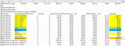
=IFERROR(INDEX('Square Input'!J$18:J$45,MATCH(1,('Square Input'!A$18:A$45="The Market")*('Square Input'!B$48:B$58=G7),0)),0)

This part of the formula needs to change -- ('Square Input'!B$48:B$58=G7) --- , but I do not know how to change it to sum up multiple totals from different cells. I'll share the image to see.

So looking at the image, I am looking at the data from rows 19-42, as it shows data from 2 locations: Market & the Blue River Lounge.
For each location, I want totals for each settlement type: Card, Cash, House Account, Gift Card. Card though has multiple lines of data, and that is my challenge. For Market, Card is a combination of rows 19-24 & row 28.

I originally had a simple formula for the sum of those specific rows but recently the system reports pulled a fast one on me and messed with the row order, so my formulas were pointed at rows not related to Card totals. For this reason I want to do an Index and Match to look at the descriptions in column B, and returning the summation of the totals in column J. I just dont know how. I'm open to ideas. I thought "hey, maybe any cell in column B with 'card' in it, but there is Gift Card which would muck up that. So I'm a bit lost for ideas and need your help.

Thank you again. It's been a very long time since I needed help and I've always come here and I'm sorry if I'm so rusty in posting that I did any of this incorrectly.
 

Attachments

  • Capture.PNG
    Capture.PNG
    87.2 KB · Views: 21

Excel Facts

Will the fill handle fill 1, 2, 3?
Yes! Type 1 in a cell. Hold down Ctrl while you drag the fill handle.
would a SUMIFS() work ???
with a LEFT(cell, 4) = "CARD"
what version of excel do you have

Row 28 - does not have card in , it has CASH APP ???

cannot see whats in G7

so you could use sumifs( using Market & CARD ) + sumifs( Market and CASH)

Note: Images are difficult to see , and also requires that I input all the data myself, which means I may make an error, which is very time consuming, and from my point of view less likely to get a response, if a complicated spreadsheet. Plus we cannot see any of the formulas used.

Therefore -

A SMALL sample spreadsheet, around 10-20 rows, would help a lot here, with all sensitive data removed, and expected results mocked up and manually entered, with a few notes of explanation.

MrExcel has a tool called “XL2BB” that lets you post samples of your data and will allow us to copy/paste your sample data into our Excel spreadsheets, saving a lot of time.

You can also test to see if it works ok, in the "Test Here" forum.

OR if you cannot get XL2BB to work, or have restrictions on your PC

then put the sample spreadsheet onto a share

I only tend to goto OneDrive, Dropbox or google docs , as I'm never certain of other random share sites and possible virus.
Please make sure you have a representative data sample and also that the data has been desensitised, remember this site is open to anyone with internet access to see - so any sensitive / personal data should be removed

Make sure you set any share or google to share to everyone
 
Upvote 0
Night Audit Spreadsheet Breck BLANK Updated.xlsx
ABCDE
1Breckenridge The Market
2Tips0.00A&G0.00
3Tax#REF!Cash0.00
4Food0.00Gift Certificate0.00
5Beverages0.00Payment Card97.51
6Merchandise0.00Room Charge16.61
7Activities0.00Voucher0.00
8Other Categories0.00Check0.00
9Credit Card Fees0.00
10Unclassified
11#REF!114.12
12
13
14
15
16Display By Location
17Filtered By Location: Blue River Lounge, The Market
18LocationPayment MethodNet Total
19The MarketCard - Dipped (Chip)$11.37
20The MarketCard - Tapped (Contactless)$86.14
21The MarketCard - Swiped$0.00
22The MarketCard - Keyed$0.00
23The MarketCard on File$0.00
24The MarketCard - Other$0.00
25The MarketCash$0.00
26The MarketGift Card$0.00
27The MarketOther$0.00
28The MarketCash App$0.00
29The MarketOpen Ticket$0.00
30The MarketHouse Account$16.61
Square Input
Cell Formulas
RangeFormula
E3:E4E3='Square Input'!C25
E5E5=SUM('Square Input'!C19:C24)+'Square Input'!C28
E6E6='Square Input'!C30
E7E7='Square Input'!C27
B2B2='Square Input'!F12
B3B3='Square Input'!#REF!
B4:B8B4=IFERROR(INDEX('Square Input'!F$31:F$34,MATCH(1,('Square Input'!A$31:A$34="The Market")*('Square Input'!B$31:B$34=A4),0)),0)
E9E9=-'Square Input'!I12
B11,E11B11=SUM(B2:B10)
 
Upvote 0
would a SUMIFS() work ???
with a LEFT(cell, 4) = "CARD"
what version of excel do you have

Row 28 - does not have card in , it has CASH APP ???

cannot see whats in G7

so you could use sumifs( using Market & CARD ) + sumifs( Market and CASH)

Note: Images are difficult to see , and also requires that I input all the data myself, which means I may make an error, which is very time consuming, and from my point of view less likely to get a response, if a complicated spreadsheet. Plus we cannot see any of the formulas used.

Therefore -

A SMALL sample spreadsheet, around 10-20 rows, would help a lot here, with all sensitive data removed, and expected results mocked up and manually entered, with a few notes of explanation.

MrExcel has a tool called “XL2BB” that lets you post samples of your data and will allow us to copy/paste your sample data into our Excel spreadsheets, saving a lot of time.

You can also test to see if it works ok, in the "Test Here" forum.

OR if you cannot get XL2BB to work, or have restrictions on your PC

then put the sample spreadsheet onto a share

I only tend to goto OneDrive, Dropbox or google docs , as I'm never certain of other random share sites and possible virus.
Please make sure you have a representative data sample and also that the data has been desensitised, remember this site is open to anyone with internet access to see - so any sensitive / personal data should be removed

Make sure you set any share or google to share to everyone

This is Office 16, from my company

Thank you! I posted teh XL2BB. I cut out a lot of the fluff to make it simple.

The top part is usually on a different tab, that is why you see 'Square Input' addressed in the formulas.

I color coordinated the cells that are related to each other. Thus, the "Payment Card" highlighted yellow is meant to have a formula that sums up all the yellow highlighted settlement types below, and so forth.

I hope this helps you out. The option I am dreading on using is a super long formula that includes a Match for each of the settlement types... in other words, a long formula summation formula that says to match "Card - Dipped (Chip)", "Card - Tapped (Contactless)" and so forth. It would be messy for sure!
 
Upvote 0
can you change the names in D2 to D9 to match the elements in B19 to B30

then you could use a SUMIF()
=SUMIF($B$19:$B$30,D3,$C$19:$C$30)
and simple refer to D2:D9 as the criteria

for the part with card then
=SUMPRODUCT((LEFT(B19:B30,4)=D5)*(C19:C30))
will add add anything that starts with card
add then you will need to add
SUMIF($B$19:$B$30,"Cash App",$C$19:$C$30)
for cash app
=SUMPRODUCT((LEFT(B19:B30,4)=D5)*(C19:C30))+SUMIF($B$19:$B$30,"Cash App",$C$19:$C$30)

otherwise , you will need to hard code the criteria
like
=SUMIF($B$19:$B$30,"house Account",$C$19:$C$30)

What are all the possible groupings
for example
Payment Card
is the Left part of all the transaction to just pull out CARD
and then we add a sumif() for "Cash App"

Cash
is everything that just has CASH as an entry only

we would probably need to see all the possibly entries and the grouping you need
perhaps in a table


Book1
ABCDE
1Breckenridge The Market
2Tips#REF!A&G0
3Tax#REF!Cash100
4Food0Gift Card111
5Beverages0Card444683429.5
6Merchandise0House Account16.61
7Activities0Voucher0
8Other Categories0Check0
9Credit Card Fees0
10Unclassified0
11#REF!0
12
13
14
15
16Display By Location
17Filtered By Location: Blue River Lounge, The Market
18LocationPayment MethodNet Total
19The MarketCard - Dipped (Chip)11.37
20The MarketCard - Tapped (Contactless)86.14
21The MarketCard - Swiped11111
22The MarketCard - Keyed222222
23The MarketCard on File2222
24The MarketCard - Other3333
25The MarketCash100
26The MarketGift Card111
27The MarketOther0
28The MarketCash App444444444
29The MarketOpen Ticket0
30The MarketHouse Account16.61
Sheet2
Cell Formulas
RangeFormula
B2B2='Square Input'!F12
B3B3='Square Input'!#REF!
B4:B8B4=IFERROR(INDEX('Square Input'!F$31:F$34,MATCH(1,('Square Input'!A$31:A$34="The Market")*('Square Input'!B$31:B$34=A4),0)),0)
B11B11=SUM(B2:B10)
E3:E4,E6:E11E3=SUMIF($B$19:$B$30,D3,$C$19:$C$30)
E5E5=SUMPRODUCT((LEFT(B19:B30,4)=D5)*(C19:C30))+SUMIF($B$19:$B$30,"Cash App",$C$19:$C$30)
 
Upvote 0
can you change the names in D2 to D9 to match the elements in B19 to B30

then you could use a SUMIF()
=SUMIF($B$19:$B$30,D3,$C$19:$C$30)
and simple refer to D2:D9 as the criteria

for the part with card then
=SUMPRODUCT((LEFT(B19:B30,4)=D5)*(C19:C30))
will add add anything that starts with card
add then you will need to add
SUMIF($B$19:$B$30,"Cash App",$C$19:$C$30)
for cash app
=SUMPRODUCT((LEFT(B19:B30,4)=D5)*(C19:C30))+SUMIF($B$19:$B$30,"Cash App",$C$19:$C$30)
Hi Etaf
This worked perfect, you are a genius! I could and did change the names in D2-9 to match the elements... Cash, Card, Gift Card, House Account, Other... That part made sense because I did the same for the revenues you see in A4-A8, but those formulas were easy to make because that part of the spreadsheet is more custom than the payment section we're dealing with.

I also used the formula given =SUMPRODUCT((LEFT(B19:B30,4)=D5)*(C19:C30))+SUMIF($B$19:$B$30,"Cash App",$C$19:$C$30) and it worked.

I need to be able to modify your formula for one additional attribute. We have 2 outlets. My XL2BB only showed "The Market" because you recommended I keep it simple, but in my actual spreadsheet directly below it is the 2nd outlet "Blue River Lounge" with exact same categories of payment types. I need to insert a Match somewhere in the formula, looking at column A "The Market" & "Blue River Lounge", but my brain isn't functioning in where I should put it.

Can I please ask for your help one last time?
 
Upvote 0
we can an extra criteria for "the market" and "Blue River Lounge"

But the you would use SUMIFS()

which has the sumrange in different postion
=SUMIFS($C$19:$C$30,$B$19:$B$30,"Cash App",$B$19:$B$30,"the market")

instead of "the market - you could use a cell reference

with
=SUMPRODUCT((LEFT(B19:B30,4)=D5)*(A19:A30="the Market")*(C19:C30))

you could have a header for "the market or Blue River

Book2
ABCDEF
1Breckenridge The Market
2The MarketBlue River Lounge
3Tips#REF!A&G0
4Tax#REF!Cash1001000
5Food0Gift Card111
6Beverages0Card444672318.511111
7Merchandise0House Account16.61
8Activities0Voucher0
9Other Categories0Check0
10Credit Card Fees0
11Unclassified0
12#REF!0
13
14
15
16
17Display By Location
18Filtered By Location: Blue River Lounge, The Market
19LocationPayment MethodNet Total
20The MarketCard - Dipped (Chip)11.37
21The MarketCard - Tapped (Contactless)86.14
22Blue River LoungeCard - Swiped11111
23The MarketCard - Keyed222222
24The MarketCard on File2222
25The MarketCard - Other3333
26The MarketCash100
27The MarketGift Card111
28Blue River LoungeCash1000
29The MarketCash App444444444
30The MarketOpen Ticket0
31The MarketHouse Account16.61
Sheet2
Cell Formulas
RangeFormula
F4F4=SUMIFS($C$20:$C$31,$B$20:$B$31,D4,$A$20:$A$31,$F$2)
F6F6=SUMPRODUCT((LEFT(B20:B31,4)=D6)*($A$20:$A$31=$F$2)*(C20:C31))+SUMIFS($C$20:$C$31,$B$20:$B$31,"Cash App",$A$20:$A$31,$F$2)
B3B3='Square Input'!F12
B4B4='Square Input'!#REF!
B5:B9B5=IFERROR(INDEX('Square Input'!F$31:F$34,MATCH(1,('Square Input'!A$31:A$34="The Market")*('Square Input'!B$31:B$34=A5),0)),0)
B12B12=SUM(B3:B11)
E4:E5,E7E4=SUMIFS($C$20:$C$31,$B$20:$B$31,D4,$A$20:$A$31,$E$2)
E6E6=SUMPRODUCT((LEFT(B20:B31,4)=D6)*($A$20:$A$31=$E$2)*(C20:C31))+SUMIFS($C$20:$C$31,$B$20:$B$31,"Cash App",$A$20:$A$31,$E$2)
E8:E12E8=SUMIF($B$20:$B$31,D8,$C$20:$C$31)


But can you perhaps post a XL2BB - with the layout of the data , so we can see best way to go and if it would be better and possible to change layout
 
Upvote 0

Forum statistics

Threads
1,215,636
Messages
6,125,961
Members
449,276
Latest member
surendra75

We've detected that you are using an adblocker.

We have a great community of people providing Excel help here, but the hosting costs are enormous. You can help keep this site running by allowing ads on MrExcel.com.
Allow Ads at MrExcel

Which adblocker are you using?

Disable AdBlock

Follow these easy steps to disable AdBlock

1)Click on the icon in the browser’s toolbar.
2)Click on the icon in the browser’s toolbar.
2)Click on the "Pause on this site" option.
Go back

Disable AdBlock Plus

Follow these easy steps to disable AdBlock Plus

1)Click on the icon in the browser’s toolbar.
2)Click on the toggle to disable it for "mrexcel.com".
Go back

Disable uBlock Origin

Follow these easy steps to disable uBlock Origin

1)Click on the icon in the browser’s toolbar.
2)Click on the "Power" button.
3)Click on the "Refresh" button.
Go back

Disable uBlock

Follow these easy steps to disable uBlock

1)Click on the icon in the browser’s toolbar.
2)Click on the "Power" button.
3)Click on the "Refresh" button.
Go back
Back
Top