VBA: Merging rows after a particular row, based off of matching entries in column

ruinedelf

New Member
Joined
Dec 6, 2023
Messages
35
Office Version
  1. 365
  2. 2021
Platform
  1. Windows
  2. MacOS
Hi all! Got another question for ya'll! This is similar to the one eiloken helped me with earlier, but it's different enough I'd like to request help here as well.

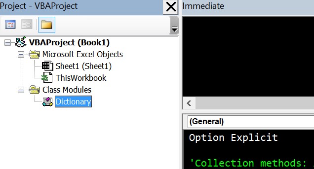
As before, the workbook needs to be OS agnostic (on both Windows and Mac at least) and as Mac does not have access to Microsoft Scripting Runtime, I'm not able to use the script I got from somewhere else that uses Dictionaries.

I have a table that looks like this:

BatchSampleAnalyte 1Analyte 2Analyte 3Analyte 4Analyte 5Analyte 6Analyte 7Analyte 8Analyte 9Analyte 10Analyte 11Analyte 12Analyte 13Analyte 14
Batch 1Sample 1<0.1<5<0.12.330.61.6<0.10.7<112.9
Batch 1Sample 140159.944050
Batch 1Sample 2<0.1<5<0.12.724.42<0.10.7<116.1
Batch 1Sample 237757.54.15190

I would like a script that would be able to merge the rows based on column B. As you can see, there are two Sample 1s and two Sample 2s, with alternating empty spots in both rows. I would like the script to be able to merge them so it would look like this:

BatchSampleAnalyte 1Analyte 2Analyte 3Analyte 4Analyte 5Analyte 6Analyte 7Analyte 8Analyte 9Analyte 10Analyte 11Analyte 12Analyte 13Analyte 14
Batch 1Sample 1<0.1<5<0.12.330.64011.6<0.159.90.74<1405012.9
Batch 1Sample 2<0.1<5<0.12.724.43772<0.157.50.74.1<1519016.1

However, there's a catch: I would like the script to only check from row 61 onwards. Anything above row 61 should not be touched.

This is the script that I have been using:
VBA Code:
Sub mergeRows()
    Const HDR As Long = 61 ' Header row
    Const col As Long = 2 ' Column used for merging rows
    Dim ws As Worksheet, lastRow As Long, i As Long
    Set ws = ThisWorkbook.Worksheets("ALS Import")
    lastRow = ws.Cells(ws.Rows.Count, col).End(xlUp).Row

    Dim ac As New Dictionary, dc As New Dictionary
    Dim itm As Variant, dRows As Range, d As Range, tr As String

    If lastRow >= HDR Then
        Application.ScreenUpdating = False

        For i = HDR To lastRow ' Find duplicate values in the chosen column
            tr = Trim(ws.Cells(i, col).Value)
            If Len(tr) > 0 Then
                If Not ac.Exists(tr) Then
                    ac.Add tr, i
                Else
                    ' If the key exists in the 'ac' dictionary, add to 'dc' for merging
                    If Not dc.Exists(ac(tr)) Then
                        dc.Add ac(tr), i
                    End If
                End If
            End If
        Next i

        For Each itm In dc ' Merge rows ---------------------------------------------------
            ' Combines rows where the chosen column values match
            For i = 1 To ws.Cells(itm, ws.Columns.Count).End(xlToLeft).Column
                If Len(Trim(ws.Cells(itm, i).Value)) = 0 Then
                    ws.Cells(itm, i).Value = ws.Cells(dc(itm), i).Value
                End If
            Next i
        Next

        For Each itm In dc ' Deletes the duplicate rows -----------------------------------
            Set d = ws.Cells(dc(itm), col)
            If dRows Is Nothing Then
                Set dRows = d
            Else
                Set dRows = Union(dRows, d)
            End If
        Next

        If Not dRows Is Nothing Then dRows.EntireRow.Delete

        Application.ScreenUpdating = True
    End If
End Sub
Hope this won't be too difficult! Thanks!
 
Give the below a try:
VBA Code:
Sub test()
    Dim x As Long, y As Long, arr1 As Variant, arr2 As Variant
    
    For x = Cells(Rows.Count, 1).End(xlUp).Row To 62 Step -1
        If Application.CountIf(Range("B62:B" & Rows.Count), Cells(x, 2)) > 1 Then
            arr1 = Range(Cells(x - 1, 3), Cells(x - 1, 16)).Value
            arr2 = Range(Cells(x, 3), Cells(x, 16)).Value
            For y = 1 To UBound(arr1, 2)
                If arr1(1, y) = "" Then arr1(1, y) = arr2(1, y)
            Next y
            Range(Cells(x - 1, 3), Cells(x - 1, 16)) = arr1
            Rows(x).EntireRow.Delete
        End If
    Next x
End Sub
 
Upvote 0

Excel Facts

Format cells as time
Select range and press Ctrl+Shift+2 to format cells as time. (Shift 2 is the @ sign).
Perhaps the below will be more dynamic, if there are a lot of rows as well as 450+ columns then performance may be a little slow. Let me know if it is and it may be better to work on the whole thing in arrays:

VBA Code:
Sub test()
    Dim x As Long, y As Long, arr1 As Variant, arr2 As Variant, lCol As Long
   
    lCol = Cells(61, Columns.Count).End(xlToLeft).Column ' header row
   
    For x = Cells(Rows.Count, 1).End(xlUp).Row To 62 Step -1
        If Application.CountIf(Range("B62:B" & Rows.Count), Cells(x, 2)) > 1 Then
            arr1 = Range(Cells(x - 1, 3), Cells(x - 1, lCol)).Value
            arr2 = Range(Cells(x, 3), Cells(x, lCol)).Value
            For y = 1 To UBound(arr1, 2)
                If arr1(1, y) = "" Then arr1(1, y) = arr2(1, y)
            Next y
            Range(Cells(x - 1, 3), Cells(x - 1, lCol)) = arr1
            Rows(x).EntireRow.Delete
        End If
    Next x
End Sub

Also, will this be used in Excel 365 only?
 
Upvote 0
Unfortunately not, it will be used on 365 and 2021 at least that I know of, maybe others, and on both Windows and Mac. Which is part of the problem, because if it was Windows only the Dictionary based script I had would've worked fine...

Remember that the Dictionary import I mentioned in the previous page is an option. There're two versions I've found:


They both throw errors at different points in the script I originally have, so it's not quite plug and play, but it still has dictionaries!

I'll give the script you've written up a spin when I get back in the office after the weekend, fingers crossed!
 
Upvote 0
I see, I will try to throw together an array only version for you to test as well. I am not a big dictionary user so will try doing it with only arrays.
 
Upvote 0
This should be a better option for working within the array, it will then remove the duplicate rows all at once at the end:
VBA Code:
Sub test()
    Dim mRng As Range, MainArr As Variant, lCol As Long, lRow As Long
    Dim x As Long, y As Long
   
    lCol = Cells(61, Columns.Count).End(xlToLeft).Column ' last used column based on header row
    lRow = Cells(Rows.Count, 1).End(xlUp).Row ' last used row based on column A
    Set mRng = Range(Cells(62, 1), Cells(lRow, lCol)) ' range of data without headers
    MainArr = mRng.Value ' pass the range to the array
   
    For x = UBound(MainArr) To 2 Step -1 ' loop through array backwards - excluding the first row
        If MainArr(x - 1, 2) = MainArr(x, 2) Then ' check if the item above in the array is the same as the current, column B
            For y = 3 To lCol ' loop through the columns, starting at column C
                If MainArr(x - 1, y) = "" Then MainArr(x - 1, y) = MainArr(x, y) ' write the blanks to the row above if they are blank
            Next y ' next column
        End If
    Next x ' next row
    mRng = MainArr ' write the array back to the range
    mRng.RemoveDuplicates 2, xlNo ' remove duplicates in range based on column B, RemoveDuplicates will always remove the bottom duplicate first
End Sub
 
Upvote 0
Solution
Thanks for the update, Georgiboy! It worked nicely on my test data at home, but I'll need to test it out on live data when I get into work after the weekend. Watch this space!
 
Upvote 0

Forum statistics

Threads
1,215,094
Messages
6,123,071
Members
449,092
Latest member
ipruravindra

We've detected that you are using an adblocker.

We have a great community of people providing Excel help here, but the hosting costs are enormous. You can help keep this site running by allowing ads on MrExcel.com.
Allow Ads at MrExcel

Which adblocker are you using?

Disable AdBlock

Follow these easy steps to disable AdBlock

1)Click on the icon in the browser’s toolbar.
2)Click on the icon in the browser’s toolbar.
2)Click on the "Pause on this site" option.
Go back

Disable AdBlock Plus

Follow these easy steps to disable AdBlock Plus

1)Click on the icon in the browser’s toolbar.
2)Click on the toggle to disable it for "mrexcel.com".
Go back

Disable uBlock Origin

Follow these easy steps to disable uBlock Origin

1)Click on the icon in the browser’s toolbar.
2)Click on the "Power" button.
3)Click on the "Refresh" button.
Go back

Disable uBlock

Follow these easy steps to disable uBlock

1)Click on the icon in the browser’s toolbar.
2)Click on the "Power" button.
3)Click on the "Refresh" button.
Go back
Back
Top