VLOOKUP Issue with Approximate Match - Need Help Categorizing Customers

happydz

New Member
Joined
Jan 11, 2017
Messages
41
I'm facing an issue with the VLOOKUP function when attempting to categorize my customers based on their values. I have a list of customer names in column A and their respective values in column B. Additionally, I have a reference table with categories in column G and their corresponding values in column H. The categories are sorted in ascending order, as follows: F (0), D (60), C (70), B (80), A (90).

I'm using the following VLOOKUP formula to categorize the customers based on their values:
=VLOOKUP(B2, G2:H6, 1, TRUE)
The problem is that when I look up for the value B2 in the range H2:H6 for the approximately value, the result was 0 although I noticed that the value of the customer (57) is near to the value in the reference table 60 for the category D.

I've double-checked my data, ensured that the cell formatting is correct, and confirmed there are no leading/trailing spaces. Despite these checks, the problem persists.

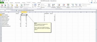
I've uploaded a screenshot of my Excel sheet to provide a clearer understanding of the issue. Any assistance or insights you can provide would be greatly appreciated.
 

Attachments

  • vlookup issue.JPG
    vlookup issue.JPG
    135.2 KB · Views: 11

Excel Facts

Copy a format multiple times
Select a formatted range. Double-click the Format Painter (left side of Home tab). You can paste formatting multiple times. Esc to stop
When using aproximate match argument as TRUE VLOOKUP will give the last record that was met. Since 57 never reaches 60 it give you 0. You can see that in other examples in your image. If you have later versions of excel the XLOOKUP and XMATCH functions have arguments that allow you to pick the next higher or next lower for the best match.

Please update your profile with what version of excel you are using so the forum can give you suggestions that fit your version.

Best Wishes.
 
Upvote 0
When using aproximate match argument as TRUE VLOOKUP will give the last record that was met. Since 57 never reaches 60 it give you 0. You can see that in other examples in your image. If you have later versions of excel the XLOOKUP and XMATCH functions have arguments that allow you to pick the next higher or next lower for the best match.

Please update your profile with what version of excel you are using so the forum can give you suggestions that fit your version.

Best Wishes.
Thank you for your reply, my Excel version is Microsoft office standard 2010. Version: 10.0.1460.1000 (32 bits)
 
Upvote 0
Then you may want to do your matching differently as 2010 doesn't go to the next value. Wrapping IFERROR around an INDEX-MATCH formula may help. But this assumes that you want the next highest number even if there is match (See 60 in this example).

It looks like you're doing a grading scale. Why not try this:

Excel Formula:
=IF(B2<=60,60,IF(B2<=70,70,IF(B2<=80,80,IF(B2<=90,90,100))))
I tried excel online google docs, but it gave the same result, however, my goal is to learn the VLOOKUP formula and the grading scale is just an example. Thank you anyway for your help. Please, keep this thread opened so that the forum may help with suggestions to use vlookup in this regard.
 
Upvote 0
Please check:

Book2
ABCDEF
1
2DataResultLookup
357600
4667060
5989070
61009080
7768090
800
96470
105560
118890
12
Sheet1
Cell Formulas
RangeFormula
C3:C11C3=IF(MIN(IF($E$3:$E$7>=$B3,$E$3:$E$7))=0,VLOOKUP($B3,$E$3:$E$7,1,1),MIN(IF($E$3:$E$7>=$B3,$E$3:$E$7)))


Thankx
Sam
 
Upvote 0
VLOOKUP is becoming more and more outdated. I suggesting using INDEX-MATCH, which is much like XLOOKUP in the newer versions of Excel, except it doesn't have the updated matching arguments.

And VLOOKUP will behave the same regardless of the version.

Finally, there are youtube channels that can really help you. Take a look at these:
Mr Excel, ExcelISFun (very comprehensive video list), Leila Gharani, and MyOnlineTrainingHub
Most have sample workbooks with before and after versions
thank you

awoohaw

 
Upvote 0
my Excel version is Microsoft office standard 2010.
Please put that information in your Account details (click your user name at the top right of the forum) so helpers always know what Excel version(s) & platform(s) you are using as the best solution often varies by version. (Don’t forget to scroll down & ‘Save’)

(57) is near to the value in the reference table 60 for the category D.
If you are looking for the closest match (up or down) then would this work for you?

23 11 05.xlsm
BCDEFGH
1DataResultCategoryValue
257DF0
366CD60
498AC70
5100AB80
676BA90
70F
864D
955D
1088A
Lookup Category
Cell Formulas
RangeFormula
C2:C10C2=INDEX(G$2:G$6,MATCH(MIN(ABS(B2-H$2:H$6)),ABS(B2-H$2:H$6),0))
Press CTRL+SHIFT+ENTER to enter array formulas.
 
Upvote 0

Forum statistics

Threads
1,215,091
Messages
6,123,062
Members
449,089
Latest member
ikke

We've detected that you are using an adblocker.

We have a great community of people providing Excel help here, but the hosting costs are enormous. You can help keep this site running by allowing ads on MrExcel.com.
Allow Ads at MrExcel

Which adblocker are you using?

Disable AdBlock

Follow these easy steps to disable AdBlock

1)Click on the icon in the browser’s toolbar.
2)Click on the icon in the browser’s toolbar.
2)Click on the "Pause on this site" option.
Go back

Disable AdBlock Plus

Follow these easy steps to disable AdBlock Plus

1)Click on the icon in the browser’s toolbar.
2)Click on the toggle to disable it for "mrexcel.com".
Go back

Disable uBlock Origin

Follow these easy steps to disable uBlock Origin

1)Click on the icon in the browser’s toolbar.
2)Click on the "Power" button.
3)Click on the "Refresh" button.
Go back

Disable uBlock

Follow these easy steps to disable uBlock

1)Click on the icon in the browser’s toolbar.
2)Click on the "Power" button.
3)Click on the "Refresh" button.
Go back
Back
Top