AVERAGEIF - single criterion in multiple columns?

[Gsaraco]

I recently became familiar with the "AVERAGEIF" function. I've gotten the hand of using it, but now I have a problem. I am working with records that can have up to five separate category codes. Thus, 5 columns are reserved for the category of a given record.

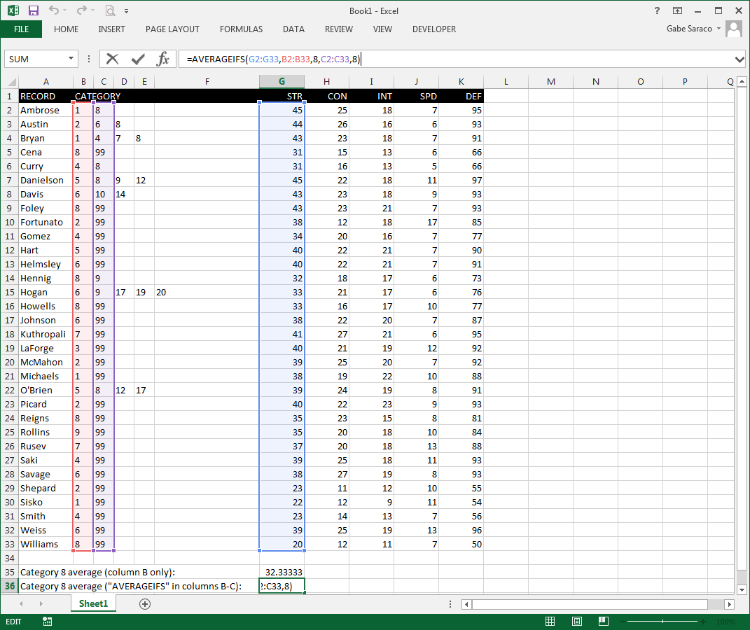
To create a column average for a specific category, I would need to include all five of those columns in the criteria range. However, when I try a range with multiple columns, Excel only seems to include rows if the code appears in the first code column. So if I need, say, a Category 8 average, and a record is both a category 1 and 8, it will be ignored because the "8" code is in the second column of my criteria range. What could I do to make Excel scan all five category columns for a given category code?

I've looked into the AVERAGEIFS function, but my understanding is that it is used when more than one criteria are present. In my situation, I only need one criterion to be included in the average - it's just that a single type of criterion is spread across multiple columns.

 

[kirbster]

Just use averageifs with the same criteria across multiple columns :-

=AVERAGEIFS(G:G,H:H,8,I:I,8,J:J,8,K:K,8,L:L,8)

Unless i've misunderstood your question

 

[Gsaraco]

Just use averageifs with the same criteria across multiple columns :-

=AVERAGEIFS(G:G,H:H,8,I:I,8,J:J,8,K:K,8,L:L,8)

Unless i've misunderstood your question

Thank you for the response! I have tried the method you described, and I always get a Divide By Zero error when I add the second criteria/range. Here is a picture to illustrate:

I tried filling all the blank cells with "99" in case that was the problem, but the Divide By Zero error persists.

 

[XOR LX]

Not sure I understand.

There doesn't appear to be a single row in your data for which both the column B and column C entries are 8, so naturally your result will be #DIV/0!.

Regards

 

[Jonmo1]

AVERAGEIFS is doing the criteria as an AND...
If B=8 AND C=8 Then average G
I believe you want OR
If B=8 OR C=8 Then average G

Can't do that with averageifs
You'll need to do a manual SUM/COUNT

Will the 8 ever appear in more than one column of the same row?
If not, try
=SUMPRODUCT((B2:E33=8)*(G2:G33))/SUMPRODUCT(--(B2:E33=8))

 

[Gsaraco]

AVERAGEIFS is doing the criteria as an AND...
If B=8 AND C=8 Then average G
I believe you want OR
If B=8 OR C=8 Then average G

Can't do that with averageifs
You'll need to do a manual SUM/COUNT

Will the 8 ever appear in more than one column of the same row?
If not, try
=SUMPRODUCT((B2:E33=8)*(G2:G33))/SUMPRODUCT(--(B2:E33=8))

Ah yes, exactly - I need a record to be in the average if 8 appears in Column B or C. 8 would never appear in more than one column.

I am going to play around with the function you suggested, thanks!

 

[Jonmo1]

You're welcome.

Just note that it's 'critical' that the 8 should never appear in more than 1 collumn for a given row.
It would cause the value in G to be averaged twice (or however many times the 8 appears in that row).

 

[Gsaraco]

You're welcome.

Just note that it's 'critical' that the 8 should never appear in more than 1 collumn for a given row.
It would cause the value in G to be averaged twice (or however many times the 8 appears in that row).

Alright, this function is doing exactly what I needed it to. Excellent.

The only snag I'm running into is that a text entry in the average range causes the formula to return a #VALUE! error.

These text entries are in certain fields in which I've used an =IF function to return a dash ('-) instead of zero, since I want them to be ignored in average calculations. This works fine for my overall averages (using a basic AVERAGE function that ignores text), but I'm wondering if there's a way to make it play nice with this SUMPRODUCT function for the purposes of my category averages.

I've tried modifying my =IF function to return no text ("") instead of the dash, but the formula still sees that as a text cell rather than a blank cell.

 

[Jonmo1]

Yep, we're not going to be able to handle the text values in the average range..

Go ahead and let your IF formulas return 0's instead of -'s
Then ammend the average to

=SUMPRODUCT((B2:E33=8)*(G2:G33))/SUMPRODUCT((B2:E33=8)*(G2:G33<>0))

 

[Aladin Akyurek]

This class of problems are better tackled with an explicit array-processing formula...

Control+shift+enter, not just enter:

=AVERAGE(IF(B2:E33=8,IF(ISNUMBER(G2:G33),G2:G33)))