TheFlyingHalibut
New Member
- Joined
- Aug 3, 2015
- Messages
- 2
Hi,
I'm having trouble with conditional formatting.
I have a large sample of data looking similar to the example below, lots of dates for lots of rows.
I am trying to use the below data to create a sort of progress bar, and initially did so by counting blank cells per row, and then in a separate sheet having a progress bar =(8-Blank Cells). Unfortunately this didn't provide me with enough information.
<tbody>
</tbody>
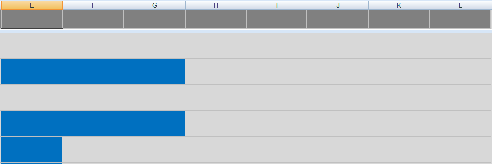
With the information above, I want to be able to represent the data similar to the image below, so it looks like progress bars against each row, however depending on how old the most recent date is, I want the progress bar to change colour.
E.g.
If the highest date within the row is less than a week old, any cell that contains data is filled blue.
If the highest date within the row is more than a week but less than two weeks old, any cell that contains data is filled yellow.
If the highest date within the row is more than two weeks old, any cell that contains data is filled orange.
I am trying to have this set up so that "raw data" is in one worksheet, and then "progress bars" are in another nice dashboard worksheet. Main reason is that I will be dumping new data into the "raw data" worksheet on the regular from some software output and do not want to have to format it to look nice each time.
Most of my formatting so far has come from nested ifs:
e.g.
 <today()-7,"c",if(data!w2,"z","")))
<today()-7,"c",if(data!ab2,"z","")))))
<today()-7,"c",if(data!ab2,"z","")))
The above example has three conditions - empty, older than a week, newer than a week.
Ideally I want a fourth condition being oldr than a week but less than two.
Please help!
Thanks,</today()-7,"c",if(data!ab2,"z","")))
</today()-7,"c",if(data!ab2,"z","")))))
</today()-7,"c",if(data!w2,"z","")))
I'm having trouble with conditional formatting.
I have a large sample of data looking similar to the example below, lots of dates for lots of rows.
I am trying to use the below data to create a sort of progress bar, and initially did so by counting blank cells per row, and then in a separate sheet having a progress bar =(8-Blank Cells). Unfortunately this didn't provide me with enough information.
| Sent | Short | Assessed | Checked | Action | Selection | Offered | Started |
| 22/06/2015 | 26/06/2015 | 28/06/2015 | 15/07/2015 | 28/07/2015 | |||
| 15/06/2015 | 17/06/2015 | 22/06/2015 | 12/07/2015 | ||||
| 14/06/2015 | 25/06/2015 | 01/07/2015 | 05/07/2015 | 01/08/2015 | 02/08/2015 | ||
| 08/06/2015 | 15/06/2015 | 20/06/2015 |
<tbody>
</tbody>
With the information above, I want to be able to represent the data similar to the image below, so it looks like progress bars against each row, however depending on how old the most recent date is, I want the progress bar to change colour.
E.g.
If the highest date within the row is less than a week old, any cell that contains data is filled blue.
If the highest date within the row is more than a week but less than two weeks old, any cell that contains data is filled yellow.
If the highest date within the row is more than two weeks old, any cell that contains data is filled orange.
I am trying to have this set up so that "raw data" is in one worksheet, and then "progress bars" are in another nice dashboard worksheet. Main reason is that I will be dumping new data into the "raw data" worksheet on the regular from some software output and do not want to have to format it to look nice each time.
Most of my formatting so far has come from nested ifs:
e.g.
<today()-7,"c",if(data!ab2,"z","")))))
<today()-7,"c",if(data!ab2,"z","")))
The above example has three conditions - empty, older than a week, newer than a week.
Ideally I want a fourth condition being oldr than a week but less than two.
Please help!
Thanks,</today()-7,"c",if(data!ab2,"z","")))
</today()-7,"c",if(data!ab2,"z","")))))
</today()-7,"c",if(data!w2,"z","")))
Last edited:


