Duplicate entries in an INDEX - based on a data validation list

[avim621]

Hi all -

So I am trying to make a finder tool within a sales organization where a salesperson can pick from a list of products (dropdown using a data validation list) and once selected, current use cases appear below that. To set that up, I used an index formula that would pull from another data table. Info/photos:

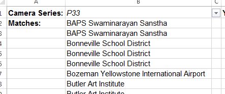
Here, you see the dropdown and the selection "P33" with the matches below that:

The formula I used to pull up the matches and is in Cell B2 above is:

=IF(ISERROR(INDEX(ProductList!$A$1:$B$1996,SMALL(IF(ProductList!$B$1:$B$1996=$B$1,ROW(ProductList!$B$1:$B$1996)),ROW(1:1)),1)),"",INDEX(ProductList!$A$1:$B$1996,SMALL(IF(ProductList!$B$1:$B$1996=$B$1,ROW(ProductList!$B$1:$B$1996)),ROW(1:1)),1))

I managed that formula from an online entry found here:

How To Return Multiple Match Values in Excel Using INDEX-MATCH or VLOOKUP | eImagine Technology Group

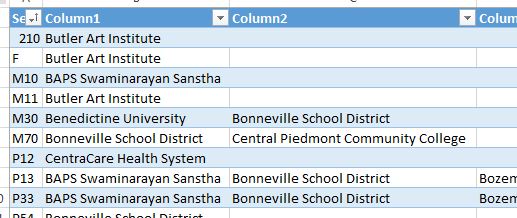
The "ProductList" worksheet referred to in that formula is:

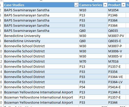
That is made on a separate worksheet. Basically, for each product, I listed the entity in additional entries so that I could list the products in their own cells.

My issue, as seen in the first photo, is that for the product "series" a broader search term, the finder is pulling up names multiple times as they have multiple products in that series.

Any thoughts on how I can code it to avoid duplicate entries in this search?

Glad to provide more info/screengrabs if needed.

Many thanks.

 

[AhoyNC]

Welcome to the forum.
Maybe something like this. Change ranges to match your data.
Instead of screen shots it is more helpful to post a small sample that can be copied into Excel, so we don't have to try and recreate your spreadsheet for testing.

The IFERROR is only in Excel ver. 2010 or later, so if you have an earlier ver. you will need to use the ISERROR as in the formula you posted.
This is an array formula and must be entered with CTRL-SHIFT-ENTER (command-return on MAC).
Formula can just be copied down as needed.

Excel Workbook
	A	B
1		P33
2	Match	BAPS
3		Bonneville
Sheet1

Excel Workbook
	A	B
1	Case	Series
2	BAPS	M10
3	BAPS	P33
4	BAPS	P33
5	University	M10
6	University	M10
7	Bonneville	P33
8	Bonneville	M10
9	Bonneville	P33
10	Bonneville	P33
ProductList

 

[avim621]

I am trying to download the Jeanie add-on but it is not functioning properly and the error message is in German.

Could you elaborate on what you did in those formulas so that I can carry it over to my current data set?

I started a new data set with listing each product only once (as I believe you suggested) and then instead listed every user following that product:

I believe this is what you were alluding to.

From there I changed my array formula to grab from this list, but I am not sure how to make the cells after it grab all of the additional entries to the right of the first one (if that makes sense).

Very thankful for your help.I am trying to download the Jeanie add-on but it is not functioning properly and the error message is in German.

Could you elaborate on what you did in those formulas so that I can carry it over to my current data set?

I started a new data set with listing each product only once (as I believe you suggested) and then instead listed every user following that product:

I believe this is what you were alluding to.

From there I changed my array formula to grab from this list, but I am not sure how to make the cells after it grab all of the additional entries to the right of the first one (if that makes sense).

Very thankful for your help.

 

[AhoyNC]

You could use HTML marker to post a sample. Here is a link which shows how to get and install it.
https://www.youtube.com/watch?v=JycvgGppxt0&feature=youtu.be

Link to English ver. of Excel Jeanie
Excel Jeanie Html

I don't think you will have to make any changes to your data base.

In my example there are 2 sheets.
Sheet 1 - Where you had Camera Series and wanted to find matches for product P33.
ProductList - database with Case Studies and Product.

If we breakdown this formula:

=IFERROR(INDEX(ProductList!$A$2:$A$10,SMALL(IF(FREQUENCY(IF(ProductList!$B$2:$B$10=$B$1,MATCH(ProductList!$A$2:$A$10,ProductList!$A$2:$A$10,0)),ROW(ProductList!$A$2:$A$10)-ROW(ProductList!$A$2)+1),ROW(ProductList!$A$2:$A$10)-ROW(ProductList!$A$2)+1),ROWS(ProductList!$A$2:A2))),"")

This part just returns an array of row numbers that are used for the BINS in the Frequency function and to return the row numbers for the INDEX

=ROW(ProductList!$A$2:$A$10)-ROW(ProductList!$A$2)+1

This returns [TABLE="width: 365"]
<colgroup><col width="365"></colgroup>[TR]
   [TD="width: 365"]{1;2;3;4;5;6;7;8;9}[/TD]
 [/TR]
[/TABLE]

The MATCH function looks at the Case Studies in the ProductList sheet and returns a row number for the matches.
So, in this example it finds BAPS in row 1, University in row 4, etc.

=MATCH(ProductList!$A$2:$A$10,ProductList!$A$2:$A$10,0)
This returns the array [TABLE="width: 365"]
<colgroup><col width="365"></colgroup>[TR]
   [TD="width: 365"]{1;1;1;4;4;6;6;6;6}[/TD]
 [/TR]
[/TABLE]

Since we only want items that match the Product in cell B2 of sheet 1 - we use the IF function

IF(ProductList!$B$2:$B$10=$B$1,MATCH(ProductList!$A$2:$A$10,ProductList!$A$2:$A$10,0))

This returns [TABLE="width: 365"]
<colgroup><col width="365"></colgroup>[TR]
   [TD="width: 365"]{FALSE;1;1;FALSE;FALSE;6;FALSE;6;6}[/TD]
 [/TR]
[/TABLE]

Since we only want unique Case Studies we use the FREQUENCY function.

FREQUENCY(IF(ProductList!$B$2:$B$10=$B$1,MATCH(ProductList!$A$2:$A$10,ProductList!$A$2:$A$10,0)),ROW(ProductList!$A$2:$A$10)-ROW(ProductList!$A$2)+1)

This returns [TABLE="width: 365"]
<colgroup><col width="365"></colgroup>[TR]
   [TD="width: 365"]{2;0;0;0;0;3;0;0;0;0}[/TD]
 [/TR]
[/TABLE]

We then use another IF to return the row numbers that match the Case Studies and product number.

IF(FREQUENCY(IF(ProductList!$B$2:$B$10=$B$1,MATCH(ProductList!$A$2:$A$10,ProductList!$A$2:$A$10,0)),ROW(ProductList!$A$2:$A$10)-ROW(ProductList!$A$2)+1),ROW(ProductList!$A$2:$A$10)-ROW(ProductList!$A$2)+1)

This returns [TABLE="width: 365"]
<colgroup><col width="365"></colgroup>[TR]
   [TD="width: 365"]{1;FALSE;FALSE;FALSE;FALSE;6;FALSE;FALSE;FALSE;FALSE}[/TD]
 [/TR]
[/TABLE]

We now have the 2 row numbers for the Case Studies (row 1 and 6).
We then use the SMALL function to return the row number to INDEX. For the "k" argument in the SMALL function we use ROWS(ProductList!$A$2:A2).

You may want to look at this link about the 16:35 min. mark. He is using FRQUENCY and MATCH to count items, but the principle is the same.
https://www.youtube.com/watch?v=ELBoMyZxBM0

Excel Workbook
	A	B
1	Find	P33
2	Match	BAPS
3		Bonneville
Sheet

Excel Workbook
	A	B
1	Case	Series
2	BAPS	M10
3	BAPS	P33
4	BAPS	P33
5	University	M10
6	University	M10
7	Bonneville	P33
8	Bonneville	M10
9	Bonneville	P33
10	Bonneville	P33
Sheet