-
If you would like to post, please check out the MrExcel Message Board FAQ and register here. If you forgot your password, you can reset your password.
You are using an out of date browser. It may not display this or other websites correctly.
You should upgrade or use an alternative browser.
You should upgrade or use an alternative browser.
Transpose or Vlookup
- Thread starter ferd109
- Start date
Excel Facts
How to fill five years of quarters?
Type 1Q-2023 in a cell. Grab the fill handle and drag down or right. After 4Q-2023, Excel will jump to 1Q-2024. Dash can be any character.
ferd109,
Welcome to the MrExcel board.
You are posting a picture. This means that if this was a problem where one needed to use your data, anyone trying to help you would have to enter the data manually. That makes no sense and I doubt you'd get any answer.
Please post a screenshot of your sheet(s), what you have and what you expect to achieve, with Excel Jeanie HTML 4 (contains graphic instructions).
http://www.excel-jeanie-html.de/html/hlp_schnell_en.php
Or, if your file does not contain sensitive information, you can upload it to www.box.net and provide a link to your workbook.
wer.
Upvote
0
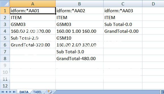
I have data in sheet as below.
$A$1:$D$9
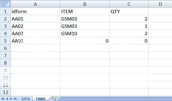
And I want to turn it into a table like in
$A$11:$D$16
<table style="font-family: Calibri,Arial; font-size: 11pt; background-color: rgb(255, 255, 255); padding-left: 2pt; padding-right: 2pt;" border="1" cellpadding="0" cellspacing="0"> <colgroup><col style="font-weight: bold; width: 30px;"><col style="width: 64px;"><col style="width: 134px;"><col style="width: 141px;"><col style="width: 114px;"></colgroup><tbody><tr style="background-color: rgb(202, 202, 202); text-align: center; font-weight: bold; font-size: 8pt;"><td>
</td><td>A</td><td>B</td><td>C</td><td>D</td></tr><tr style="height: 18px;"><td style="font-size: 8pt; background-color: rgb(202, 202, 202); text-align: center;">1</td><td>
</td><td>A</td><td>B</td><td>C</td></tr><tr style="height: 18px;"><td style="font-size: 8pt; background-color: rgb(202, 202, 202); text-align: center;">2</td><td style="text-align: right;">1</td><td>idform:*AA01</td><td>idform:*AA02</td><td>idform:*AA03</td></tr><tr style="height: 18px;"><td style="font-size: 8pt; background-color: rgb(202, 202, 202); text-align: center;">3</td><td style="text-align: right;">2</td><td>ITEM</td><td>ITEM</td><td>ITEM</td></tr><tr style="height: 18px;"><td style="font-size: 8pt; background-color: rgb(202, 202, 202); text-align: center;">4</td><td style="text-align: right;">3</td><td>GSM03</td><td>GSM03</td><td>Sub Total-0.0</td></tr><tr style="height: 18px;"><td style="font-size: 8pt; background-color: rgb(202, 202, 202); text-align: center;">5</td><td style="text-align: right;">4</td><td>160.00 2.00 320.00</td><td>160.00 1.00 160.00</td><td>GrandTotal-0.00</td></tr><tr style="height: 18px;"><td style="font-size: 8pt; background-color: rgb(202, 202, 202); text-align: center;">6</td><td style="text-align: right;">5</td><td>Sub Total-2.0</td><td>GSM10</td><td>
</td></tr><tr style="height: 18px;"><td style="font-size: 8pt; background-color: rgb(202, 202, 202); text-align: center;">7</td><td style="text-align: right;">6</td><td>GrandTotal-320.00</td><td>160.00 2.00 320.00</td><td>
</td></tr><tr style="height: 18px;"><td style="font-size: 8pt; background-color: rgb(202, 202, 202); text-align: center;">8</td><td style="text-align: right;">7</td><td>
</td><td>Sub Total-3.0</td><td>
</td></tr><tr style="height: 18px;"><td style="font-size: 8pt; background-color: rgb(202, 202, 202); text-align: center;">9</td><td style="text-align: right;">8</td><td>
</td><td>GrandTotal-480.00</td><td>
</td></tr><tr style="height: 18px;"><td style="font-size: 8pt; background-color: rgb(202, 202, 202); text-align: center;">10</td><td style="background-color: rgb(150, 150, 150);">
</td><td style="background-color: rgb(150, 150, 150);">
</td><td style="background-color: rgb(150, 150, 150);">
</td><td style="background-color: rgb(150, 150, 150);">
</td></tr><tr style="height: 18px;"><td style="font-size: 8pt; background-color: rgb(202, 202, 202); text-align: center;">11</td><td>
</td><td>A</td><td>B</td><td>C</td></tr><tr style="height: 18px;"><td style="font-size: 8pt; background-color: rgb(202, 202, 202); text-align: center;">12</td><td style="text-align: right;">1</td><td>idform</td><td>ITEM</td><td>QTY</td></tr><tr style="height: 18px;"><td style="font-size: 8pt; background-color: rgb(202, 202, 202); text-align: center;">13</td><td style="text-align: right;">2</td><td>AA01</td><td>GSM03</td><td style="text-align: right;">2</td></tr><tr style="height: 18px;"><td style="font-size: 8pt; background-color: rgb(202, 202, 202); text-align: center;">14</td><td style="text-align: right;">3</td><td>AA02</td><td>GSM03</td><td style="text-align: right;">1</td></tr><tr style="height: 18px;"><td style="font-size: 8pt; background-color: rgb(202, 202, 202); text-align: center;">15</td><td style="text-align: right;">4</td><td>AA02</td><td>GSM10</td><td style="text-align: right;">2</td></tr><tr style="height: 18px;"><td style="font-size: 8pt; background-color: rgb(202, 202, 202); text-align: center;">16</td><td style="text-align: right;">5</td><td>AA03</td><td style="text-align: right;">0</td><td style="text-align: right;">0</td></tr></tbody></table>
What is the formula used tranpose?
$A$1:$D$9
And I want to turn it into a table like in
$A$11:$D$16
<table style="font-family: Calibri,Arial; font-size: 11pt; background-color: rgb(255, 255, 255); padding-left: 2pt; padding-right: 2pt;" border="1" cellpadding="0" cellspacing="0"> <colgroup><col style="font-weight: bold; width: 30px;"><col style="width: 64px;"><col style="width: 134px;"><col style="width: 141px;"><col style="width: 114px;"></colgroup><tbody><tr style="background-color: rgb(202, 202, 202); text-align: center; font-weight: bold; font-size: 8pt;"><td>
</td><td>A</td><td>B</td><td>C</td><td>D</td></tr><tr style="height: 18px;"><td style="font-size: 8pt; background-color: rgb(202, 202, 202); text-align: center;">1</td><td>
</td><td>A</td><td>B</td><td>C</td></tr><tr style="height: 18px;"><td style="font-size: 8pt; background-color: rgb(202, 202, 202); text-align: center;">2</td><td style="text-align: right;">1</td><td>idform:*AA01</td><td>idform:*AA02</td><td>idform:*AA03</td></tr><tr style="height: 18px;"><td style="font-size: 8pt; background-color: rgb(202, 202, 202); text-align: center;">3</td><td style="text-align: right;">2</td><td>ITEM</td><td>ITEM</td><td>ITEM</td></tr><tr style="height: 18px;"><td style="font-size: 8pt; background-color: rgb(202, 202, 202); text-align: center;">4</td><td style="text-align: right;">3</td><td>GSM03</td><td>GSM03</td><td>Sub Total-0.0</td></tr><tr style="height: 18px;"><td style="font-size: 8pt; background-color: rgb(202, 202, 202); text-align: center;">5</td><td style="text-align: right;">4</td><td>160.00 2.00 320.00</td><td>160.00 1.00 160.00</td><td>GrandTotal-0.00</td></tr><tr style="height: 18px;"><td style="font-size: 8pt; background-color: rgb(202, 202, 202); text-align: center;">6</td><td style="text-align: right;">5</td><td>Sub Total-2.0</td><td>GSM10</td><td>
</td></tr><tr style="height: 18px;"><td style="font-size: 8pt; background-color: rgb(202, 202, 202); text-align: center;">7</td><td style="text-align: right;">6</td><td>GrandTotal-320.00</td><td>160.00 2.00 320.00</td><td>
</td></tr><tr style="height: 18px;"><td style="font-size: 8pt; background-color: rgb(202, 202, 202); text-align: center;">8</td><td style="text-align: right;">7</td><td>
</td><td>Sub Total-3.0</td><td>
</td></tr><tr style="height: 18px;"><td style="font-size: 8pt; background-color: rgb(202, 202, 202); text-align: center;">9</td><td style="text-align: right;">8</td><td>
</td><td>GrandTotal-480.00</td><td>
</td></tr><tr style="height: 18px;"><td style="font-size: 8pt; background-color: rgb(202, 202, 202); text-align: center;">10</td><td style="background-color: rgb(150, 150, 150);">
</td><td style="background-color: rgb(150, 150, 150);">
</td><td style="background-color: rgb(150, 150, 150);">
</td><td style="background-color: rgb(150, 150, 150);">
</td></tr><tr style="height: 18px;"><td style="font-size: 8pt; background-color: rgb(202, 202, 202); text-align: center;">11</td><td>
</td><td>A</td><td>B</td><td>C</td></tr><tr style="height: 18px;"><td style="font-size: 8pt; background-color: rgb(202, 202, 202); text-align: center;">12</td><td style="text-align: right;">1</td><td>idform</td><td>ITEM</td><td>QTY</td></tr><tr style="height: 18px;"><td style="font-size: 8pt; background-color: rgb(202, 202, 202); text-align: center;">13</td><td style="text-align: right;">2</td><td>AA01</td><td>GSM03</td><td style="text-align: right;">2</td></tr><tr style="height: 18px;"><td style="font-size: 8pt; background-color: rgb(202, 202, 202); text-align: center;">14</td><td style="text-align: right;">3</td><td>AA02</td><td>GSM03</td><td style="text-align: right;">1</td></tr><tr style="height: 18px;"><td style="font-size: 8pt; background-color: rgb(202, 202, 202); text-align: center;">15</td><td style="text-align: right;">4</td><td>AA02</td><td>GSM10</td><td style="text-align: right;">2</td></tr><tr style="height: 18px;"><td style="font-size: 8pt; background-color: rgb(202, 202, 202); text-align: center;">16</td><td style="text-align: right;">5</td><td>AA03</td><td style="text-align: right;">0</td><td style="text-align: right;">0</td></tr></tbody></table>
What is the formula used tranpose?
Upvote
0
ferd109,
Per your original graphic.
Is this what you actual raw data looks like in sheet "DATA"?
Is this what your actual new table looks like in sheet "TABEL"?
Per your original graphic.
Is this what you actual raw data looks like in sheet "DATA"?
| Excel Workbook | |||||
|---|---|---|---|---|---|
| A | B | C | |||
| 1 | idform:*AA01 | idform:*AA02 | idform:*AA03 | ||
| 2 | ITEM | ITEM | ITEM | ||
| 3 | GSM03 | GSM03 | Sub Total-0.0 | ||
| 4 | 160.00 2.00 320.00 | 160.00 1.00 160.00 | GrandTotal-0.00 | ||
| 5 | Sub Total-2.0 | GSM10 | |||
| 6 | GrandTotal-320.00 | 160.00 2.00 320.00 | |||
| 7 | Sub Total-3.0 | ||||
| 8 | GrandTotal-480.00 | ||||
| 9 | |||||
DATA | |||||
Is this what your actual new table looks like in sheet "TABEL"?
| Excel Workbook | |||||
|---|---|---|---|---|---|
| A | B | C | |||
| 1 | idform | ITEM | QTY | ||
| 2 | AA01 | GSM03 | 2 | ||
| 3 | AA02 | GSM03 | 1 | ||
| 4 | AA02 | GSM10 | 2 | ||
| 5 | AA03 | 0 | 0 | ||
| 6 | |||||
TABEL | |||||
Upvote
0
jbeaucaire
Well-known Member
- Joined
- May 8, 2002
- Messages
- 6,012
I would have to use a macro to do it:
========
How to use the macro:
1. Open up your workbook
2. Get into VB Editor (Press Alt+F11)
3. Insert a new module (Insert > Module)
4. Copy and Paste in your code (given above)
5. Get out of VBA (Press Alt+Q)
6. Save your sheet
The macro is installed and ready to use. Press Alt-F8 and select it from the macro list.
==============
Code:
Option Explicit
Option Compare Text

Sub ReFormatData()
'JBeaucaire  (11/5/2009)
Dim LR As Long, LC As Long, NR As Long, i As Long, r As Long
Dim MyArr, MyStr As String

LC = Cells(1, Columns.Count).End(xlToLeft).Column
LR = Range("A1").SpecialCells(xlCellTypeLastCell).Row
NR = LR + 2

Range("A" & LR + 1, "C" & LR + 1).Interior.ColorIndex = 24
Range("A" & LR + 2) = "IDFORM"
Range("B" & LR + 2) = "ITEM"
Range("C" & LR + 2) = "QTY"

For i = 1 To LC
    MyStr = Replace(Cells(1, i), "idform:*", "")
    For r = 2 To LR
    Select Case Left(Cells(r, i), 4)
        Case "ITEM"
            NR = NR + 1
            Range("A" & NR) = MyStr
            r = r + 1
            If Not Left(Cells(r, i), 3) = "Sub" And Not Left(Cells(r, i), 3) = "Gra" Then
                Range("B" & NR) = Cells(r, i)
                If IsNumeric(Left(Cells(r + 1, i), 1)) Then
                    MyArr = Split(Cells(r + 1, i), " ")
                    Range("C" & NR) = MyArr(1)
                Else
                    Range("B" & NR, "C" & NR) = 0
                End If
            End If
            r = r + 1
        Case "Sub ", "Gran", ""
            Exit For
        Case Else
            NR = NR + 1
            Range("A" & NR) = MyStr
            If Not Left(Cells(r, i), 3) = "Sub" And Not Left(Cells(r, i), 3) = "Gra" Then
                Range("B" & NR) = Cells(r, i)
                If IsNumeric(Left(Cells(r + 1, i), 1)) Then
                    MyArr = Split(Cells(r + 1, i), " ")
                    Range("C" & NR) = MyArr(1)
                End If
            Else
                Range("B" & NR, "C" & NR) = 0
            End If
            r = r + 1
        End Select
    Next r
Next i
End SubHow to use the macro:
1. Open up your workbook
2. Get into VB Editor (Press Alt+F11)
3. Insert a new module (Insert > Module)
4. Copy and Paste in your code (given above)
5. Get out of VBA (Press Alt+Q)
6. Save your sheet
The macro is installed and ready to use. Press Alt-F8 and select it from the macro list.
==============
| Excel Workbook | |||||||||||
|---|---|---|---|---|---|---|---|---|---|---|---|
| A | B | C | D | E | F | G | H | I | |||
| 1 | idform:*AA01 | idform:*AA02 | idform:*AA03 | idform:*AA04 | idform:*AA05 | idform:*AA06 | idform:*AA07 | idform:*AA08 | idform:*AA09 | ||
| 2 | ITEM | ITEM | ITEM | ITEM | ITEM | ITEM | ITEM | ITEM | ITEM | ||
| 3 | GSM03 | GSM03 | Sub Total-0.0 | GSM03 | GSM03 | Sub Total-0.0 | GSM03 | GSM03 | Sub Total-0.0 | ||
| 4 | 160.00 2.00 320.00 | 160.00 1.00 160.00 | GrandTotal-0.00 | 160.00 2.00 320.00 | 160.00 1.00 160.00 | GrandTotal-0.00 | 160.00 2.00 320.00 | 160.00 1.00 160.00 | GrandTotal-0.00 | ||
| 5 | Sub Total-2.0 | GSM10 | Sub Total-2.0 | GSM10 | Sub Total-2.0 | GSM10 | |||||
| 6 | GrandTotal-320.00 | 160.00 2.00 320.00 | GrandTotal-320.00 | 160.00 2.00 320.00 | GrandTotal-320.00 | 160.00 2.00 320.00 | |||||
| 7 | Sub Total-3.0 | Sub Total-3.0 | Sub Total-3.0 | ||||||||
| 8 | GrandTotal-480.00 | GrandTotal-480.00 | GrandTotal-480.00 | ||||||||
BEFORE | |||||||||||
| Excel Workbook | |||||
|---|---|---|---|---|---|
| A | B | C | |||
| 9 | |||||
| 10 | IDFORM | ITEM | QTY | ||
| 11 | AA01 | GSM03 | 2 | ||
| 12 | AA02 | GSM03 | 1 | ||
| 13 | AA02 | GSM10 | 2 | ||
| 14 | AA03 | ||||
| 15 | AA04 | GSM03 | 2 | ||
| 16 | AA05 | GSM03 | 1 | ||
| 17 | AA05 | GSM10 | 2 | ||
| 18 | AA06 | ||||
| 19 | AA07 | GSM03 | 2 | ||
| 20 | AA08 | GSM03 | 1 | ||
| 21 | AA08 | GSM10 | 2 | ||
| 22 | AA09 | ||||
AFTER | |||||
Last edited:
Upvote
0
ferd109,
With two worksheets in your workbook, the raw data is in sheet "DATA", and the other worksheet is "TABEL". And, the macro will work with more than the three columns you displayed.
Before the macro:
After the macro:
Please TEST this FIRST in a COPY of your workbook (always make a backup copy before trying new code, you never know what you might lose).
Adding the Macro
1. Copy the below macro, by highlighting the macro code and pressing the keys CTRL + C
2. Open your workbook
3. Press the keys ALT + F11 to open the Visual Basic Editor
4. Press the keys ALT + I to activate the Insert menu
5. Press M to insert a Standard Module
6. Paste the code by pressing the keys CTRL + V
7. Press the keys ALT + Q to exit the Editor, and return to Excel
8. To run the macro from Excel, open the workbook, and press ALT + F8 to display the Run Macro Dialog. Double Click the macro's name to Run it.
Then run the "MoveData" macro.
With two worksheets in your workbook, the raw data is in sheet "DATA", and the other worksheet is "TABEL". And, the macro will work with more than the three columns you displayed.
Before the macro:
| Excel Workbook | |||||
|---|---|---|---|---|---|
| A | B | C | |||
| 1 | idform:*AA01 | idform:*AA02 | idform:*AA03 | ||
| 2 | ITEM | ITEM | ITEM | ||
| 3 | GSM03 | GSM03 | Sub Total-0.0 | ||
| 4 | 160.00 2.00 320.00 | 160.00 1.00 160.00 | GrandTotal-0.00 | ||
| 5 | Sub Total-2.0 | GSM10 | |||
| 6 | GrandTotal-320.00 | 160.00 2.00 320.00 | |||
| 7 | Sub Total-3.0 | ||||
| 8 | GrandTotal-480.00 | ||||
| 9 | |||||
DATA | |||||
| Excel Workbook | |||||
|---|---|---|---|---|---|
| A | B | C | |||
| 1 | |||||
| 2 | |||||
| 3 | |||||
| 4 | |||||
| 5 | |||||
| 6 | |||||
TABEL | |||||
After the macro:
| Excel Workbook | |||||
|---|---|---|---|---|---|
| A | B | C | |||
| 1 | idform | Item | QTY | ||
| 2 | AA01 | GSM03 | 2 | ||
| 3 | AA02 | GSM03 | 1 | ||
| 4 | AA03 | GSM10 | 2 | ||
| 5 | AA03 | 0 | 0 | ||
| 6 | |||||
TABEL | |||||
Please TEST this FIRST in a COPY of your workbook (always make a backup copy before trying new code, you never know what you might lose).
Adding the Macro
1. Copy the below macro, by highlighting the macro code and pressing the keys CTRL + C
2. Open your workbook
3. Press the keys ALT + F11 to open the Visual Basic Editor
4. Press the keys ALT + I to activate the Insert menu
5. Press M to insert a Standard Module
6. Paste the code by pressing the keys CTRL + V
7. Press the keys ALT + Q to exit the Editor, and return to Excel
8. To run the macro from Excel, open the workbook, and press ALT + F8 to display the Run Macro Dialog. Double Click the macro's name to Run it.
Code:
Option Explicit
Sub MoveData()
Dim ws1 As Worksheet, ws2 As Worksheet
Dim c As Range, firstaddress As String, Sp
Dim LR As Long, LC As Long, NC As Long, NR As Long, a As Long, b As Long, rng As Range
Dim Myidform As String
Application.ScreenUpdating = False
Set ws1 = Worksheets("DATA")
Set ws2 = Worksheets("TABEL")
With ws2
  .Cells.ClearContents
  .Range("A1").Resize(, 3).Value = [{"idform","Item","QTY"}]
End With
ws1.Select
With ws1
  LC = .Cells(1, Columns.Count).End(xlToLeft).Column
  For NC = 1 To LC Step 1
    NR = ws2.Cells(Rows.Count, 1).End(xlUp).Row + 1
    Myidform = Right(.Cells(1, NC), Len(.Cells(1, NC)) - WorksheetFunction.Find("*", .Cells(1, NC), 1))
    Set rng = .Columns(NC)
    a = Application.WorksheetFunction.CountIf(rng, "GSM*")
    ws2.Range("A" & NR & ":A" & NR + a - 1) = Myidform
    If a = 0 Then
      ws2.Range("B" & NR) = 0
      ws2.Range("C" & NR) = 0
    Else
      With .Columns(NC)
        Set c = .Find("GSM*", LookIn:=xlValues, LookAt:=xlWhole)
        If Not c Is Nothing Then
          firstaddress = c.Address
          Do
            ws2.Range("B" & NR) = c
            Sp = Split(c.Offset(1), " ")
            ws2.Range("C" & NR) = Sp(1)
            NR = NR + 1
            Set c = .FindNext(c)
          Loop While Not c Is Nothing And c.Address <> firstaddress
        End If
      End With
    End If
  Next NC
End With
ws2.Select
Application.ScreenUpdating = True
End Sub
Then run the "MoveData" macro.
Upvote
0
hiker.. thanks for u'r support..
<table style="font-family: Arial,Arial; font-size: 10pt; background-color: rgb(255, 255, 255); padding-left: 2pt; padding-right: 2pt;" border="1" cellpadding="0" cellspacing="0"> <colgroup><col style="font-weight: bold; width: 30px;"><col style="width: 64px;"><col style="width: 64px;"><col style="width: 64px;"></colgroup><tbody><tr style="background-color: rgb(202, 202, 202); text-align: center; font-weight: bold; font-size: 8pt;"><td>
</td><td>A</td><td>B</td><td>C</td></tr><tr style="height: 17px;"><td style="font-size: 8pt; background-color: rgb(202, 202, 202); text-align: center;">1</td><td>idform</td><td>Item</td><td>QTY</td></tr><tr style="height: 17px;"><td style="font-size: 8pt; background-color: rgb(202, 202, 202); text-align: center;">2</td><td>AA01</td><td>GSM03</td><td style="text-align: right;">2</td></tr><tr style="height: 17px;"><td style="font-size: 8pt; background-color: rgb(202, 202, 202); text-align: center;">3</td><td>AA02</td><td>GSM03</td><td style="text-align: right;">1</td></tr><tr style="height: 17px;"><td style="font-size: 8pt; background-color: rgb(202, 202, 202); text-align: center;">4</td><td>AA03</td><td>GSM10</td><td style="text-align: right;">2</td></tr><tr style="height: 17px;"><td style="font-size: 8pt; background-color: rgb(202, 202, 202); text-align: center;">5</td><td>AA03</td><td style="text-align: right;">0</td><td style="text-align: right;">0</td></tr><tr style="height: 17px;"><td style="font-size: 8pt; background-color: rgb(202, 202, 202); text-align: center;">6</td><td>
</td><td>
</td><td>
</td></tr></tbody></table>
but result A4 should AA02
so for macro.. what i must change...
tq be4..
Upvote
0
ferd109,
My mistake for not checking the output.
Before the macro:
After the updated macro:
Please TEST this FIRST in a COPY of your workbook (always make a backup copy before trying new code, you never know what you might lose).
Then run the "MoveData" macro.
My mistake for not checking the output.
Before the macro:
| Excel Workbook | |||||
|---|---|---|---|---|---|
| A | B | C | |||
| 1 | idform:*AA01 | idform:*AA02 | idform:*AA03 | ||
| 2 | ITEM | ITEM | ITEM | ||
| 3 | GSM03 | GSM03 | Sub Total-0.0 | ||
| 4 | 160.00 2.00 320.00 | 160.00 1.00 160.00 | GrandTotal-0.00 | ||
| 5 | Sub Total-2.0 | GSM10 | |||
| 6 | GrandTotal-320.00 | 160.00 2.00 320.00 | |||
| 7 | Sub Total-3.0 | ||||
| 8 | GrandTotal-480.00 | ||||
| 9 | |||||
DATA | |||||
| Excel Workbook | |||||
|---|---|---|---|---|---|
| A | B | C | |||
| 1 | |||||
| 2 | |||||
| 3 | |||||
| 4 | |||||
| 5 | |||||
| 6 | |||||
TABEL | |||||
After the updated macro:
| Excel Workbook | |||||
|---|---|---|---|---|---|
| A | B | C | |||
| 1 | idform | Item | QTY | ||
| 2 | AA01 | GSM03 | 2 | ||
| 3 | AA02 | GSM03 | 1 | ||
| 4 | AA02 | GSM10 | 2 | ||
| 5 | AA03 | 0 | 0 | ||
| 6 | |||||
TABEL | |||||
Please TEST this FIRST in a COPY of your workbook (always make a backup copy before trying new code, you never know what you might lose).
Code:
Option Explicit
Sub MoveData()
Dim ws1 As Worksheet, ws2 As Worksheet
Dim c As Range, firstaddress As String, Sp
Dim LR As Long, LC As Long, NC As Long, NR As Long, a As Long, b As Long, rng As Range
Dim Myidform As String
Application.ScreenUpdating = False
Set ws1 = Worksheets("DATA")
Set ws2 = Worksheets("TABEL")
With ws2
  .Cells.ClearContents
  .Range("A1").Resize(, 3).Value = [{"idform","Item","QTY"}]
End With
ws1.Select
With ws1
  LC = .Cells(1, Columns.Count).End(xlToLeft).Column
  For NC = 1 To LC Step 1
    NR = ws2.Cells(Rows.Count, 1).End(xlUp).Row + 1
    Myidform = Right(.Cells(1, NC), Len(.Cells(1, NC)) - WorksheetFunction.Find("*", .Cells(1, NC), 1))
    Set rng = .Columns(NC)
    a = Application.WorksheetFunction.CountIf(rng, "GSM*")
    If a = 0 Then
      ws2.Range("A" & NR) = Myidform
      ws2.Range("B" & NR) = 0
      ws2.Range("C" & NR) = 0
    Else
      ws2.Range("A" & NR & ":A" & NR + a - 1) = Myidform
      With .Columns(NC)
        Set c = .Find("GSM*", LookIn:=xlValues, LookAt:=xlWhole)
        If Not c Is Nothing Then
          firstaddress = c.Address
          Do
            ws2.Range("B" & NR) = c
            Sp = Split(c.Offset(1), " ")
            ws2.Range("C" & NR) = Sp(1)
            NR = NR + 1
            Set c = .FindNext(c)
          Loop While Not c Is Nothing And c.Address <> firstaddress
        End If
      End With
    End If
  Next NC
End With
ws2.Select
Application.ScreenUpdating = True
End Sub
Then run the "MoveData" macro.
Upvote
0
Similar threads
- Replies
- 1
- Views
- 366
- Replies
- 6
- Views
- 285
- Replies
- 14
- Views
- 266
- Replies
- 3
- Views
- 91


