a conditional format tweak for icons

John Caines

Well-known Member
Joined
Aug 28, 2006
Messages
1,155
Office Version
  1. 2019
Platform
  1. Windows
Hello All.
I have a formula in cell P5 which is;
Code:
=IF(M5="Completed",1,0)
In cell M5 there is a drop down menu which says;
Code:
Not Started
Just Started
In Progress
On Hold
Cancelled

COMPLETED

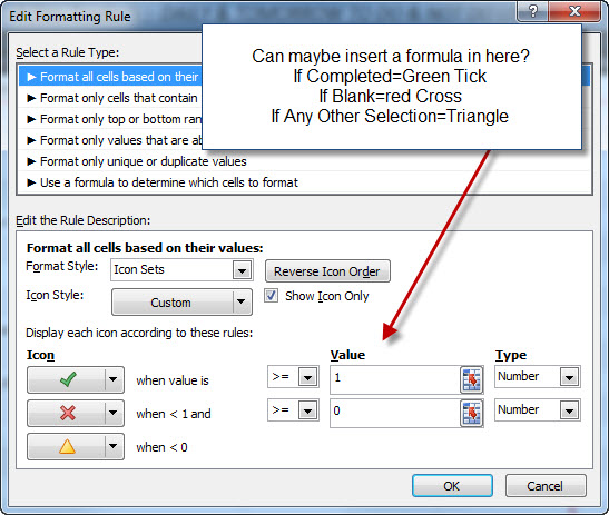
I got this from a google video about excel,, and managed to make Cell P5 show either a TICK Icon Or A CROSS icon,,from the conditional formatting/icon sets.
Tick is set at >=1 Type is Number
CROSS is set at >=0 Type is Number.

My question is,,,
How can I alter the formulas so I can show 3 different Icons in Cell P5?

A Tick If "Completed" is selected in M5
A Cross If M5 is Blank
A Triangle If It doesn't equal any of the above 2,, so basically if
Not Started
Just Started
In Progress
On Hold
Cancelled
are selected.

I've tried googling,, I can't seem to find how to do this.

I hope someone can advise.
many Thanks
JC
 

Excel Facts

What do {} around a formula in the formula bar mean?
{Formula} means the formula was entered using Ctrl+Shift+Enter signifying an old-style array formula.
Just to add,,
Do I ned the formula in Cell P5?????????
Which is,
Code:
=IF(M5="Completed",1,0)

Can it be achieved by just using formulas in the icon sets & reference M5 (Drop down words)??
See attached
TLWFz.jpg


Not sure what the formula would be :(
 
Upvote 0
I came across another forum post here;
http://www.mrexcel.com/forum/showthread.php?t=589125

This now gives me 3 of the icons to use.
code is;
Code:
=MATCH(M5,{"Cancelled","In Progress","Completed"},0)
Thing is,,
1.. If the drop downs don't equal any of the above 3,, I get #N/A showing in my cells :(
2.. Anyway to teak the above formula so that with "In progress" I can add;

"Just Started"
"On Hold"

???????
I did just try and guess,,, failed miserably :(
Code:
MATCH((M5,("Cancelled" ("In Progress","Just Started","On Hold"),"Completed"),0),"")
Just an Idea,,,might be somewhere near?????????

Many Thanks
JC
 
Upvote 0
Just tried this; Excel accepted the formula,, but it didn't work :(
Must be near?????????
Code:
MATCH((M5,("Cancelled" ("In Progress"OR"Just Started"OR"On Hold"),"Completed"),0),"")

Any ideas anybody please...
many Thanks
JC

I love excel!! (When it works,, or shall I say, I get it to work) :)
 
Upvote 0
Sorry,,, I'm wrong Totally!!!!!!!!!!!!!!
it didn't accept it,,, I just didn't have the = sign in the formula bar!!!!!!!!!!!

:(
I need a coffee. :(
 
Upvote 0
I still can't get this!!! ......
maybe I haven't explained it to well.
Let me try again,,, with no fluff. :)
=============================
I have a spreadsheet.
In Column M (M5:M44) each cell has a dropdown list that says;
Code:
Not Started
Just Started
In Progress
On Hold
Cancelled

COMPLETED
In Column P (P5:P44) I would like each cell to display1 of 3 different icons
via conditional formatting,, depending on what word has been selected
from the drop down list mentioned above. If M cell is Blank (No Icon)

3 conditions I'd like would be:

ICON Set (Green Tick) If "COMPLETED" is selected.
ICON Set (Goldish Triangle) If any of "Not Started" or "Just Started"
or "In Progress" or "On Hold" are selected
ICON Set (Red Cross) If "Cancelled" Is Selected


That's it.
I just don't know how to write the formula for the corresponding P Cells,
Or in the conditional formatting,, if these need formulas,, what they would be.
(Maybe they don't need a formula in the conditional formatting? Depends i suppose on the formula used in the P cells?

If somebody can help me it really would be a great help.
It's really really stumped me.

I just need the 3 icons applied to the 6 items mentioned in the dropdown list.
Help Please!!! :)

many thanks again
JC
 
Upvote 0
In P5 your formula would be =IF(M5="Cancelled",3,IF(M5="Completed",4,2))

Your Conditional formating would be > 3 for the Green check
Your Conditional formating would be > 2 for the Red X
Your Conditional formating would be <=2 for the Yellow triangle


What did you want if M5 were blank?
 
Upvote 0
Many Thanks again for your reply Charlie45,,

I really was struggling with this.
I did recently post on another forum for an answer,, here,, (for cross posting purposes. here's the link..
http://www.excelforum.com/excel-general/814595-use-3-icons-in-conditional-formatting-by-formula.html

A guy called Rory replied.
(OnErrorGoto0)
I saw this reply before I saw that you have replied here Charlie45
I tried his example sheet,, it seems to all work fine,,
he done it slightly differently though.

Code:
=IFERROR(MATCH(A8,$F$2:$F$7,0),"")
This was in his example sheet,, with the F range showing the dropdown words I'd want to use.
My formula now is;
Code:
=IFERROR(MATCH(M5,'DTL-To Do-2011-v4n.xlsm'!Status,0),"")
I'm not 100% sure if I inserted the name from the name manager correctly,,,,,,,,,,,,,
###AS I'M TYPING THIS I JUST TRIED SOMTHING,,IT WORKED,,,,:)
Formula now is;
Code:
=IFERROR(MATCH(M5,Status,0),"")
Ok,, great stuff.
This seems to work fine,, & leaves blanks, IE no icon showing if a blank is selected.

I'll probably stick with Rory's code Charlie45.
Again,, many thanks for your help,, really appreciate it.
I'm sure your IF formula,, I can use elsewhere soon... I can now see how you combine 2 IF's together.

All the best,, and thanks again,,

A very grateful
John Caines
 
Upvote 0

Forum statistics

Threads
1,215,637
Messages
6,125,963
Members
449,276
Latest member
surendra75

We've detected that you are using an adblocker.

We have a great community of people providing Excel help here, but the hosting costs are enormous. You can help keep this site running by allowing ads on MrExcel.com.
Allow Ads at MrExcel

Which adblocker are you using?

Disable AdBlock

Follow these easy steps to disable AdBlock

1)Click on the icon in the browser’s toolbar.
2)Click on the icon in the browser’s toolbar.
2)Click on the "Pause on this site" option.
Go back

Disable AdBlock Plus

Follow these easy steps to disable AdBlock Plus

1)Click on the icon in the browser’s toolbar.
2)Click on the toggle to disable it for "mrexcel.com".
Go back

Disable uBlock Origin

Follow these easy steps to disable uBlock Origin

1)Click on the icon in the browser’s toolbar.
2)Click on the "Power" button.
3)Click on the "Refresh" button.
Go back

Disable uBlock

Follow these easy steps to disable uBlock

1)Click on the icon in the browser’s toolbar.
2)Click on the "Power" button.
3)Click on the "Refresh" button.
Go back
Back
Top