bunkermentality
New Member
- Joined
- Sep 27, 2022
- Messages
- 4
- Office Version
- 2013
- Platform
- Windows
I'm trying to create what seems to me should be a simple task. But I'm failing badly. I suspect that my underlying data has the wrong design.
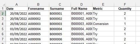
My source data "Playing Metric"s is a list of scorers from a series of rugby matches. Scores are called Try, Conversion and Penalty. Values are Try = 5, Conversion =2 and Penalty = 3.
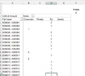
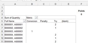
On the pivot sheet I can see the total scores per player but I want to add a calculated column F with formula Try*5+Conversion*2+Penalty*3. Try as I might I cannot make this happen.
Any advice would be most welcome
My source data "Playing Metric"s is a list of scorers from a series of rugby matches. Scores are called Try, Conversion and Penalty. Values are Try = 5, Conversion =2 and Penalty = 3.
On the pivot sheet I can see the total scores per player but I want to add a calculated column F with formula Try*5+Conversion*2+Penalty*3. Try as I might I cannot make this happen.
Any advice would be most welcome
| Ealing 1871 Training and Playing Records 2022-23.xlsx | ||||||||
|---|---|---|---|---|---|---|---|---|
| A | B | C | D | E | F | |||
| 1 | Date | Forename | Surname | Full Name | Metric | Amount | ||
| 2 | 20/08/2022 | A000001 | B000001 | B000001, A000001 | Try | 2 | ||
| 3 | 20/08/2022 | A000002 | B000002 | B000002, A000002 | Try | 1 | ||
| 4 | 20/08/2022 | A000003 | B000003 | B000003, A000003 | Conversion | 1 | ||
| 5 | 03/09/2022 | A000004 | B000004 | B000004, A000004 | Try | 2 | ||
| 6 | 03/09/2022 | A000005 | B000005 | B000005, A000005 | Try | 1 | ||
| 7 | 03/09/2022 | A000006 | B000006 | B000006, A000006 | Try | 2 | ||
| 8 | 03/09/2022 | A000007 | B000007 | B000007, A000007 | Try | 1 | ||
| 9 | 03/09/2022 | A000008 | B000008 | B000008, A000008 | Try | 2 | ||
| 10 | 03/09/2022 | A000009 | B000009 | B000009, A000009 | Try | 1 | ||
| 11 | 03/09/2022 | A000010 | B000010 | B000010, A000010 | Conversion | 5 | ||
| 12 | 03/09/2022 | A000011 | B000011 | B000011, A000011 | Try | 1 | ||
| 13 | 03/09/2022 | A000012 | B000012 | B000012, A000012 | Conversion | 2 | ||
| 14 | 03/09/2022 | A000013 | B000013 | B000013, A000013 | Try | 1 | ||
| 15 | 03/09/2022 | A000014 | B000014 | B000014, A000014 | Try | 1 | ||
| 16 | 03/09/2022 | A000015 | B000015 | B000015, A000015 | Try | 1 | ||
| 17 | 03/09/2022 | A000016 | B000016 | B000016, A000016 | Try | 1 | ||
| 18 | 03/09/2022 | A000017 | B000017 | B000017, A000017 | Try | 1 | ||
| 19 | 03/09/2022 | A000018 | B000018 | B000018, A000018 | Conversion | 1 | ||
| 20 | 03/09/2022 | A000019 | B000019 | B000019, A000019 | Conversion | 2 | ||
| 21 | 10/09/2022 | A000020 | B000020 | B000020, A000020 | Try | 2 | ||
| 22 | 10/09/2022 | A000021 | B000021 | B000021, A000021 | Try | 3 | ||
| 23 | 10/09/2022 | A000022 | B000022 | B000022, A000022 | Try | 1 | ||
| 24 | 10/09/2022 | A000023 | B000023 | B000023, A000023 | Conversion | 1 | ||
| 25 | 10/09/2022 | A000024 | B000024 | B000024, A000024 | Conversion | 6 | ||
| 26 | 10/09/2022 | A000025 | B000025 | B000025, A000025 | Penalty | 3 | ||
| 27 | 10/09/2022 | A000026 | B000026 | B000026, A000026 | Try | 1 | ||
| 28 | 10/09/2022 | A000027 | B000027 | B000027, A000027 | Try | 1 | ||
| 29 | 10/09/2022 | A000028 | B000028 | B000028, A000028 | Try | 1 | ||
| 30 | 10/09/2022 | A000029 | B000029 | B000029, A000029 | Try | 1 | ||
| 31 | 10/09/2022 | A000030 | B000030 | B000030, A000030 | Conversion | 2 | ||
| 32 | 10/09/2022 | A000031 | B000031 | B000031, A000031 | Try | 1 | ||
| 33 | 10/09/2022 | A000032 | B000032 | B000032, A000032 | Try | 1 | ||
| 34 | 17/09/2022 | A000033 | B000033 | B000033, A000033 | Penalty | 1 | ||
| 35 | 17/09/2022 | A000034 | B000034 | B000034, A000034 | Try | 1 | ||
| 36 | 17/09/2022 | A000035 | B000035 | B000035, A000035 | Conversion | 1 | ||
| 37 | 17/09/2022 | A000036 | B000036 | B000036, A000036 | Try | 1 | ||
| 38 | 17/09/2022 | A000037 | B000037 | B000037, A000037 | Try | 1 | ||
| 39 | 17/09/2022 | A000038 | B000038 | B000038, A000038 | Conversion | 1 | ||
| 40 | 17/09/2022 | A000039 | B000039 | B000039, A000039 | Penalty | 3 | ||
| 41 | 17/09/2022 | A000040 | B000040 | B000040, A000040 | Try | 1 | ||
| 42 | 17/09/2022 | A000041 | B000041 | B000041, A000041 | Try | 1 | ||
| 43 | 17/09/2022 | A000042 | B000042 | B000042, A000042 | Try | 1 | ||
| 44 | 17/09/2022 | A000043 | B000043 | B000043, A000043 | Try | 1 | ||
| 45 | 17/09/2022 | A000044 | B000044 | B000044, A000044 | Try | 1 | ||
| 46 | 17/09/2022 | A000045 | B000045 | B000045, A000045 | Conversion | 7 | ||
| 47 | 17/09/2022 | A000046 | B000046 | B000046, A000046 | Penalty | 2 | ||
Playing Metrics | ||||||||
| Cell Formulas | ||
|---|---|---|
| Range | Formula | |
| D2:D47 | D2 | =CONCATENATE(C2&", "&B2) |
| Ealing 1871 Training and Playing Records 2022-23.xlsx | ||||||||
|---|---|---|---|---|---|---|---|---|
| A | B | C | D | E | F | |||
| 1 | ||||||||
| 2 | Points | |||||||
| 3 | 0 | |||||||
| 4 | SUM of Amount | Metric | ||||||
| 5 | Full Name | Conversion | Penalty | Try | (blank) | |||
| 6 | B000001, A000001 | 2 | ||||||
| 7 | B000002, A000002 | 1 | ||||||
| 8 | B000003, A000003 | 1 | ||||||
| 9 | B000004, A000004 | 2 | ||||||
| 10 | B000005, A000005 | 1 | ||||||
| 11 | B000006, A000006 | 2 | ||||||
| 12 | B000007, A000007 | 1 | ||||||
| 13 | B000008, A000008 | 2 | ||||||
| 14 | B000009, A000009 | 1 | ||||||
| 15 | B000010, A000010 | 5 | ||||||
| 16 | B000011, A000011 | 1 | ||||||
| 17 | B000012, A000012 | 2 | ||||||
| 18 | B000013, A000013 | 1 | ||||||
| 19 | B000014, A000014 | 1 | ||||||
| 20 | B000015, A000015 | 1 | ||||||
| 21 | B000016, A000016 | 1 | ||||||
| 22 | B000017, A000017 | 1 | ||||||
| 23 | B000018, A000018 | 1 | ||||||
| 24 | B000019, A000019 | 2 | ||||||
| 25 | B000020, A000020 | 2 | ||||||
| 26 | B000021, A000021 | 3 | ||||||
| 27 | B000022, A000022 | 1 | ||||||
| 28 | B000023, A000023 | 1 | ||||||
| 29 | B000024, A000024 | 6 | ||||||
| 30 | B000025, A000025 | 3 | ||||||
| 31 | B000026, A000026 | 1 | ||||||
| 32 | B000027, A000027 | 1 | ||||||
| 33 | B000028, A000028 | 1 | ||||||
| 34 | B000029, A000029 | 1 | ||||||
| 35 | B000030, A000030 | 2 | ||||||
| 36 | B000031, A000031 | 1 | ||||||
| 37 | B000032, A000032 | 1 | ||||||
| 38 | B000033, A000033 | 1 | ||||||
| 39 | B000034, A000034 | 1 | ||||||
| 40 | B000035, A000035 | 1 | ||||||
| 41 | B000036, A000036 | 1 | ||||||
| 42 | B000037, A000037 | 1 | ||||||
| 43 | B000038, A000038 | 1 | ||||||
| 44 | B000039, A000039 | 3 | ||||||
| 45 | B000040, A000040 | 1 | ||||||
| 46 | B000041, A000041 | 1 | ||||||
| 47 | B000042, A000042 | 1 | ||||||
| 48 | B000043, A000043 | 1 | ||||||
| 49 | B000044, A000044 | 1 | ||||||
| 50 | B000045, A000045 | 7 | ||||||
| 51 | B000046, A000046 | 2 | ||||||
| 52 | (blank) | |||||||
| 53 | Grand Total | 29 | 9 | 38 | ||||
Playing Metrics Pivot | ||||||||
| Cell Formulas | ||
|---|---|---|
| Range | Formula | |
| F3 | F3 | =D3*5+B3*2+C3*3 |
")


