Automatically add thick border?

LionelHutz

New Member
Joined
Apr 1, 2015
Messages
40
Hi, hopefully I explain this well...

I have data in cells A2:P2. This data goes down about 100 rows so far. I currently have all cells with a thin border. However when the value in column B changes, I want the entire bottom border to change to a thick outline. So it would look something like this:
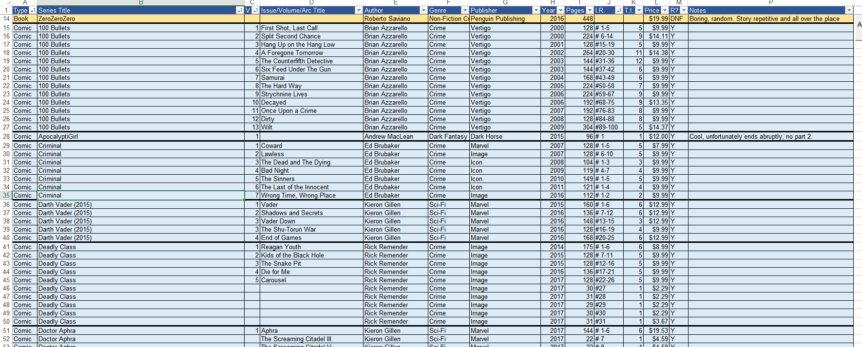
Capture.png


I tried conditional formatting by selecting the area I want it to be applicable, then using formula =$B2<>$B3. This works in theory but I cannot chose thick lines as an option for format. Is there a VBA code or macro I can use to accomplish the same?

Thanks!
 

Excel Facts

Show numbers in thousands?
Use a custom number format of #,##0,K. Each comma after the final 0 will divide the displayed number by another thousand
Not sure what you mean when you say I have data in A2 to P2

So you only want border to change in column "B"

So if the value in C45 changes you want a border put around B45 is that what you want?
 
Last edited:
Upvote 0
Maybe this

Code:
Sub MM1()
 Dim lr As Long, r As Long
 lr = Cells(Rows.Count, "B").End(xlUp).Row
 For r = 2 To lr
    If Range("B" & r) <> Range("B" & r - 1) Then
        With Range("A" & r & ":P" & r).Borders(xlEdgeBottom)
            .LineStyle = xlContinuous
            .Weight = xlThick
        End With
        With Range("A" & r & ":P" & r).Borders(xlEdgeTop)
            .LineStyle = xlContinuous
            .Weight = xlThick
        End With
    End If
Next r
End Sub
 
Upvote 0
You said:
when the value in column B changes
.

So only if a value in column B changes? Or if any cell in Column B to P changes put a bottom border on that cell.

If that is what you want try this:

This is an auto sheet event script
Your Workbook must be Macro enabled
To install this code:
Right-click on the sheet tab
Select View Code from the pop-up context menu
Paste the code in the VBA edit window


Code:
Private Sub Worksheet_Change(ByVal Target As Range)
'Modified 2-4-18 5:25 PM EST
Dim Lastrow As Long
Lastrow = Cells(Rows.Count, "A").End(xlUp).Row
If Not Intersect(Target, Range("A2:P" & Lastrow)) Is Nothing Then
If Target.Cells.Count > 1 Or IsEmpty(Target) Then Exit Sub
    With Target.Borders(xlEdgeBottom)
        .LineStyle = xlContinuous
        .Weight = xlMedium
    End With
End If
End Sub
 
Upvote 0
...
I tried conditional formatting by selecting the area I want it to be applicable, then using formula =$B2<>$B3. This works in theory but I cannot chose thick lines as an option for format. Is there a VBA code or macro I can use to accomplish the same?
.

How about normally formatting all the cells with a thick border and then use Conditional Formatting to put a thin border when =($B2=$B3)
 
Upvote 0
Hi MAIT
I read this
when the value in column B changes
to mean when the values are different, not when they actively change....we shall see ..;)
 
Upvote 0
Wow! Awesome idea lol. Super simple and very clever! Worked perfectly!
Hi Pal,
I am trying to do the same exercise. I have a huge amount of data in a table with several columns, where one column "D" includes almost 102 countries, and in which some are repeated in different rows, I need to simply group these countries each with a thick border please. I couldn't even figure out how I can do this using "Conditional formatting". Would highly appreciate any help in this matter. Thanks in advance!
 
Upvote 0

Forum statistics

Threads
1,223,445
Messages
6,172,177
Members
452,446
Latest member
walkman99

We've detected that you are using an adblocker.

We have a great community of people providing Excel help here, but the hosting costs are enormous. You can help keep this site running by allowing ads on MrExcel.com.
Allow Ads at MrExcel

Which adblocker are you using?

Disable AdBlock

Follow these easy steps to disable AdBlock

1)Click on the icon in the browser’s toolbar.
2)Click on the icon in the browser’s toolbar.
2)Click on the "Pause on this site" option.
Go back

Disable AdBlock Plus

Follow these easy steps to disable AdBlock Plus

1)Click on the icon in the browser’s toolbar.
2)Click on the toggle to disable it for "mrexcel.com".
Go back

Disable uBlock Origin

Follow these easy steps to disable uBlock Origin

1)Click on the icon in the browser’s toolbar.
2)Click on the "Power" button.
3)Click on the "Refresh" button.
Go back

Disable uBlock

Follow these easy steps to disable uBlock

1)Click on the icon in the browser’s toolbar.
2)Click on the "Power" button.
3)Click on the "Refresh" button.
Go back
Back
Top