Complex Excel formula to return results from other pages within a spreadsheet

[washhousescott]

I am trying to format a formula that will search for the last value in a column, then check to see if the corresponding value in a different column of the same row matches a given parameter. If it does, then I want to display the last value from the column, if it does not then I want it to show nothing. For example:

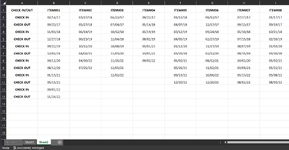
Sheet 1 has a list of Items from different sheets in the same workbook, Sheet 2 displays these items across columns and each item has Check In/Out dates. I want a formula on Sheet1 for each item that will perform the above action for each item on Sheet2. I have used various bots and have come close. The following formula, =INDEX('Sheet2'!B:B,COUNTA('Sheet2'!B:B)) , will always return the last value in the column but does not check for the "Date In" parameter. This formula, =IF(INDEX('Sheet2'!A:A,MATCH("Date In",'Sheet2'!A:A,0))="Date In",INDEX('Sheet2-GC'!B:B,MATCH("Date In",'Sheet2'!A:A,0)),"") checks for the "Date In" value first so will always return the first Check In date, not the latest.

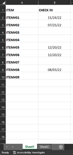
The first attached image is an example of Sheet2, the second is what I expect the formula to accomplish.

Any assistance would be greatly appreciated.

 

[Eric W]

Welcome to the MrExcel forum!

If you only have 2 values in column A, you can try this:

Book1
	A	B	C	D	E	F	G	H
1	Check In/Out	ITEM#01	ITEM#02	ITEM#03			ITEM	Check Out
2	Check In	2/14/2017	3/27/2018	4/22/2017			ITEM#01	11/24/2022
3	Check Out	9/23/2017	5/27/2018	7/4/2017			ITEM#02	7/25/2022
4	Check In	11/3/2018	6/14/2019	10/12/2018			ITEM#03
5	Check Out	12/27/2018	6/23/2019	12/4/2018
6	Check In	9/22/2019	10/11/2020	10/8/2019
7	Check Out	12/2/2019	4/2/2021	11/3/2020
8	Check In	4/12/2020	4/30/2012	11/25/2021
9	Check Out	8/12/2020	7/25/2022	12/3/2021
10	Check In	1/15/2021		12/2/2022
11	Check Out	5/15/2021
12	Check In	9/1/2022
13	Check Out	11/24/2022
14
15
Sheet1

Cell Formulas
Range	Formula
H2:H4	H2	=LET(f,FILTER($B$2:$D$20,$B$1:$D$1=G2),IF(MOD(SUM(SIGN(f)),2)=0,MAX(f),""))

 

[washhousescott]

Thanks for replying! I simplified the spread sheet a bit. It actually includes a row for the name of the person who checked out the item.

Territory Example.xlsx
	A	B	C	D	E
1	CHECK IN/OUT	ITEM#01	ITEM#02	ITEM#03	ITEM#04
2	NAME	J. SMITH	J. SMITH	J. SMITH	J. SMITH
3	CHECK IN	02/14/17	03/27/18	04/22/17	09/22/17
4	CHECK OUT	09/23/17	05/27/18	07/04/17	05/14/18
5	NAME	J. SMITH	J. SMITH	J. SMITH	J. SMITH
6	CHECK IN	11/03/18	06/14/19	10/12/18	05/19/19
7	CHECK OUT	12/27/18	06/23/19	12/04/18	08/02/19
8	NAME	J. SMITH	J. SMITH	J. SMITH	J. SMITH
9	CHECK IN	09/22/19	10/11/20	10/08/19	05/01/21
10	CHECK OUT	12/02/19	04/02/21	11/03/20	10/01/21
11	NAME	J. SMITH	J. SMITH	J. SMITH	J. SMITH
12	CHECK IN	04/12/20	04/30/22	11/25/21	09/02/22
13	CHECK OUT	08/12/20	07/25/22	12/03/21
14	NAME	J. SMITH	J. SMITH	J. SMITH
15	CHECK IN	01/15/21		12/02/22
16	CHECK OUT	05/15/21
17	NAME	J. SMITH
18	CHECK IN	09/01/22
19	CHECK OUT	11/24/22
Sheet2

 

[Eric W]

I'm not sure if that actually makes it simpler. Good spreadsheet design usually suggests that there should only be one type of data in each column. Otherwise formulas referencing that column have to take into account multiple types of data, and that makes them more complicated. However, from a usability standpoint, maybe it makes it easier for you to work with, and in this case the formula doesn't have to change much:

Book1
	A	B	C	D	E	F	G	H
1	CHECK IN/OUT	ITEM#01	ITEM#02	ITEM#03	ITEM#04		ITEM	Check Out
2	NAME	J. SMITH	J. SMITH	J. SMITH	J. SMITH		ITEM#01	11/24/2022
3	CHECK IN	2/14/2017	3/27/2018	4/22/2017	9/22/2017		ITEM#02	7/25/2022
4	CHECK OUT	9/23/2017	5/27/2018	7/4/2017	5/14/2018		ITEM#03
5	NAME	J. SMITH	J. SMITH	J. SMITH	J. SMITH		ITEM#04
6	CHECK IN	11/3/2018	6/14/2019	10/12/2018	5/19/2019
7	CHECK OUT	12/27/2018	6/23/2019	12/4/2018	8/2/2019
8	NAME	J. SMITH	J. SMITH	J. SMITH	J. SMITH
9	CHECK IN	9/22/2019	10/11/2020	10/8/2019	5/1/2021
10	CHECK OUT	12/2/2019	4/2/2021	11/3/2020	10/1/2021
11	NAME	J. SMITH	J. SMITH	J. SMITH	J. SMITH
12	CHECK IN	4/12/2020	4/30/2022	11/25/2021	9/2/2022
13	CHECK OUT	8/12/2020	7/25/2022	12/3/2021
14	NAME	J. SMITH	J. SMITH	J. SMITH
15	CHECK IN	1/15/2021		12/2/2022
16	CHECK OUT	5/15/2021
17	NAME	J. SMITH
18	CHECK IN	9/1/2022
19	CHECK OUT	11/24/2022
20
Sheet1

Cell Formulas
Range	Formula
H2:H5	H2	=LET(f,INDEX($B$2:$E$20,0,MATCH(G2,$B$1:$E$1,0)),IF(MOD(COUNT(f),2)=0,MAX(f),""))

 

[washhousescott]

I'm sorry, I meant I simplified it for my first post. The second is an accurate reproduction. Would this formula update dynamically as more dates are added to each column?

 

[Eric W]

It's a good idea to make your question as close to your actual situation as possible. Even a small difference can make an answer not work right.

And yes, the formula will update dynamically as you add more dates, as long as you make the first range include as many blank rows at the end as you think you may need, $B$2:$E$200 for example. Change the E column to include all the ITEMs you have, and you can leave blank columns there too.

 

[washhousescott]

Thanks so much for your help! I hate to bother you, but if I wanted a similar formula, but wanted to match the DATE OUT value in column A, how would I adjust the formula?

 

[Eric W]

I'm confused. There isn't a DATE OUT value in column A. If you mean CHECK OUT, that's is what already is out. Have you changed the layout of your sheet? If so, what does it look like now?

 

[washhousescott]

I am so sorry! I created a redacted version of one of the sheets and was not paying attention to the IN/OUT column. I have included the actual layout of the sheet. I will say, even though the IN/OUT rows were switched previously, the formula you provided still worked. I'm not sure why since I don't understand the formula, but I appreciate your time and assistance regardless. The formula I mentioned for the OUT value is because I want to perform a check to see if a particular item has been checked out for longer than a set period of time (3 months). If so, then it would only need to return the date the item was checked out, otherwise it would be blank. I would like to pair that with a formula to return the name of the person who last checked out the item, if possible.

I understand I am asking for a lot, and would not be upset if I need to look elsewhere for this level of assistance.

Territory Example.xlsx
	A	B	C	D	E	F	G	H	I
1	DATE IN/OUT	ITEM#01	ITEM#02	ITEM#03	ITEM#04	ITEM#05	ITEM#06	ITEM#07	ITEM#08
2	NAME	J. SMITH	J. SMITH	J. SMITH	J. SMITH	J. SMITH	J. SMITH	J. SMITH	J. SMITH
3	DATE OUT	02/14/17	03/27/18	04/22/17	09/22/17	01/12/18	09/12/17	07/27/17	01/17/17
4	DATE IN	09/23/17	05/27/18	07/04/17	05/14/18	04/07/18	12/17/17	09/13/17	09/19/17
5	NAME	J. SMITH	J. SMITH	J. SMITH	J. SMITH	J. SMITH	J. SMITH	J. SMITH	J. SMITH
6	DATE OUT	11/03/18	06/14/19	10/12/18	05/19/19	03/12/19	09/24/18	05/10/18	10/21/18
7	DATE IN	12/27/18	06/23/19	12/04/18	08/02/19	04/05/19	02/27/19	07/15/18	02/26/19
8	NAME	J. SMITH	J. SMITH	J. SMITH	J. SMITH	J. SMITH	J. SMITH	J. SMITH	J. SMITH
9	DATE OUT	09/22/19	10/11/20	10/08/19	05/01/21	01/12/20	11/17/19	08/07/19	01/03/20
10	DATE IN	12/02/19	04/02/21	11/03/20	10/01/21	03/20/20	02/12/20	09/15/19	03/10/20
11	NAME	J. SMITH	J. SMITH	J. SMITH	J. SMITH	J. SMITH	J. SMITH	J. SMITH	J. SMITH
12	DATE OUT	04/12/20	04/30/22	11/25/21	09/02/22	05/02/21	08/12/21	10/02/20	05/02/21
13	DATE IN	08/12/20	07/25/22	12/03/21		05/26/21	11/02/21	03/09/21	05/22/21
14	NAME	J. SMITH		J. SMITH		J. SMITH	J. SMITH	J. SMITH	J. SMITH
15	DATE OUT	01/15/21		12/02/22		09/13/22	10/06/22	05/13/22	05/08/22
16	DATE IN	05/15/21				12/20/22	12/20/22		08/03/22
17	NAME	J. SMITH
18	DATE OUT	09/01/22
19	DATE IN	11/24/22
Sheet2