Conditional Counting + Comparison

[klosheen]

Hi,

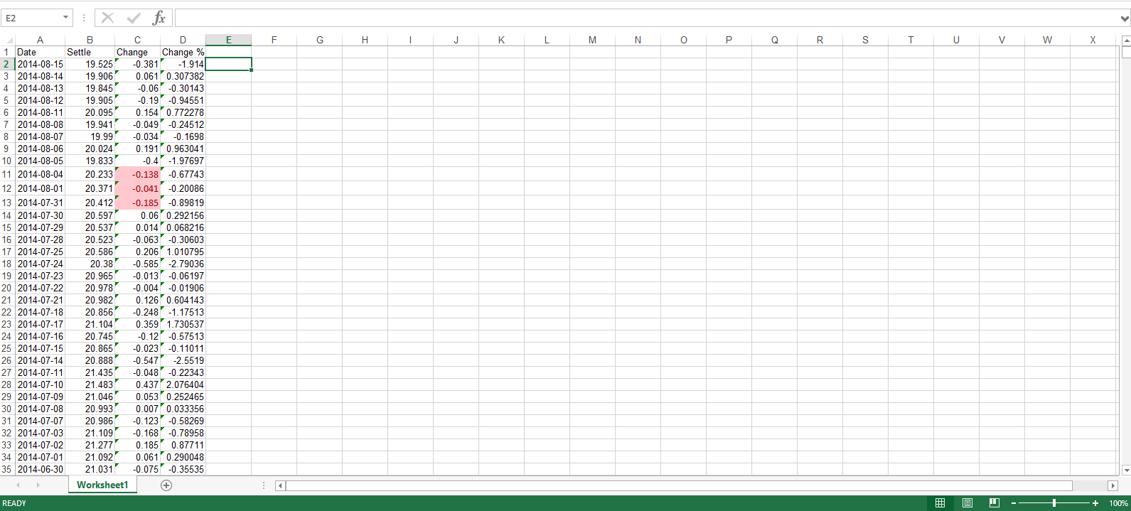
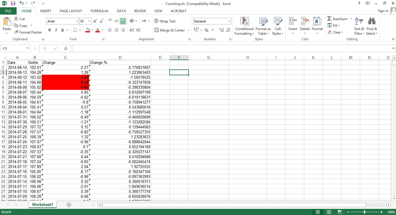
Below is a table with the daily settlment price for ICE Brent Futures. Highlighted in red are three consecutive days on which Brent finished in the red. I would like to be able to find the last time Brent suffered three consecutive daily losses or more. In other words, I would like to be able to make statements similar to the following: "This is Brent's longest losing streak since the [# of days] ended [date]."

Many thanks for all your help in advance.

 

[klosheen]

finding the negative numbers is done automatically by a formula in a helper column, other helper columns find each "negative run length". So if current negative run = 4 you only need to find the last time a run of 3 occurred - this is very easy to do - but is it what you want?

If the current negative run = 4, then I'll need to find the last time a run of 4 or more occurred.

 

[XOR LX]

I have tried copying and pasting to mimic what oldbrewer did, but the formatting turns out all jumbled up.

Here's a link to the Excel file https://drive.google.com/file/d/0Bw3-U7VqHHqAYjVVSUlLODY4VG8/edit?usp=sharing

Cheers.

Thanks, though I'm not sure which are your expected results in there?

Regards

 

[klosheen]

Thanks, though I'm not sure which are your expected results in there?

Regards

I highlighted three consecutive days on which the instrument finished lower (from 31/07 to 04/08). I want to find out the last time such a negative run was either matched or surpassed - i.e. the last time the instrument finished lower three days in a row or more.

Cheers.

 

[XOR LX]

Thanks, but why doesn't that run of 3 you've highlighted (which I presume you intend to indicate the most recent) go from 01/08/2014 to 05/08/2014?

Really not sure, but perhaps something like this array formula**, which, when copied down, will give the most recent dates in a series of three for which the change is negative for all three:

=IFERROR(INDEX(A:A,SMALL(IF(COUNTIF(OFFSET($C$2,ROW($C$2:$C$6379)-MIN(ROW($C$2:$C$6379)),,3,),"<0")=3,ROW($C$2:$C$6379)),ROWS($1:1))),"")

Regards


**Array formulas are not entered in the same way as 'standard' formulas. Instead of pressing just ENTER, you first hold down CTRL and SHIFT, and only then press ENTER. If you've done it correctly, you'll notice Excel puts curly brackets {} around the formula (though do not attempt to manually insert these yourself).</SPAN></SPAN>

 

[oldbrewer]

problem with link = just copy first 10 rows and just paste into here

 

[klosheen]

Thanks, but why doesn't that run of 3 you've highlighted (which I presume you intend to indicate the most recent) go from 01/08/2014 to 05/08/2014?

Really not sure, but perhaps something like this array formula**, which, when copied down, will give the most recent dates in a series of three for which the change is negative for all three:

=IFERROR(INDEX(A:A,SMALL(IF(COUNTIF(OFFSET($C$2,ROW($C$2:$C$6379)-MIN(ROW($C$2:$C$6379)),,3,),"<0")=3,ROW($C$2:$C$6379)),ROWS($1:1))),"")

Regards


**Array formulas are not entered in the same way as 'standard' formulas. Instead of pressing just ENTER, you first hold down CTRL and SHIFT, and only then press ENTER. If you've done it correctly, you'll notice Excel puts curly brackets {} around the formula (though do not attempt to manually insert these yourself).

Thanks. I just missed the negative reading on 05/08. The array formula you've provided shows the most recent run of three negative values. I was looking for the time before that. Also, I don't know how to adjust it to look for larger negative or positive runs. Maybe this is something that could be done more easily with R.

All the same, many thanks for your time and effort. It's really appreciated. Wish there was something I could do to help you.

 

[XOR LX]

Thanks. I just missed the negative reading on 05/08. The array formula you've provided shows the most recent run of three negative values. I was looking for the time before that. Also, I don't know how to adjust it to look for larger negative or positive runs. Maybe this is something that could be done more easily with R.

All the same, many thanks for your time and effort. It's really appreciated. Wish there was something I could do to help you.

Re-read my last post, in particular the part about copying the formula down. The 3 is the part that you need to amend, so better still to make it an actual cell reference, e.g. G1, and play about with values in there:

=IFERROR(INDEX(A:A,SMALL(IF(COUNTIF(OFFSET($C$2,ROW($C$2:$C$6379)-MIN(ROW($C$2:$C$6379)),,$G$1,),"<0")=$G$1,ROW($C$2:$C$6379)),ROWS($1:1))),"")

Regards

 

[klosheen]

Re-read my last post, in particular the part about copying the formula down. The 3 is the part that you need to amend, so better still to make it an actual cell reference, e.g. G1, and play about with values in there:

=IFERROR(INDEX(A:A,SMALL(IF(COUNTIF(OFFSET($C$2,ROW($C$2:$C$6379)-MIN(ROW($C$2:$C$6379)),,$G$1,),"<0")=$G$1,ROW($C$2:$C$6379)),ROWS($1:1))),"")

Regards

Thanks mate. It works like a charm, but only for negative values. I tried changing the <0 to >0, but it did not work.

 

[XOR LX]

Thanks mate. It works like a charm, but only for negative values. I tried changing the <0 to >0, but it did not work.

You didn't say anything about positive values?!

It should work fine with the change you made - perhaps you can update the link to your attachment with your attempt in?

Cheers

 

[klosheen]

You didn't say anything about positive values?!

It should work fine with the change you made - perhaps you can update the link to your attachment with your attempt in?

Cheers

Here's a link to the updated file: https://drive.google.com/file/d/0Bw3-U7VqHHqANlJVOUVRLVRqbWs/edit?usp=sharing