Formula for adding up minutes

[Nelly3007]

Hello,

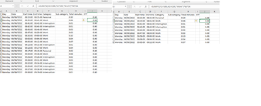
I have got a log of minutes and each set of minutes has a category. I want to add up the minutes for each category at the top of the sheet as you can see. I thought a SUM would work and have tried '=SUMIFS(F2:F100,H2:H100,"Work")' - this seems to know they are minutes but also brings up 0:00:00. Any suggestions please?

Thank you

 

[JamesCanale]

I'll bet that you want:

=SUMIFS(f2:f100,h2:h100,"Work")*60*24

And format it as a number, not a time.

It's all about how excel deals with dates and times.

 

[Nelly3007]

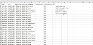
Thanks for you reply, however, this still brings up zero on all cells; I have tried the 'minutes' column formatted as minutes and number, the 'total' cells formatted as minutes and number, still the same result . Also tried the formula the other way round in case I had done it wrong. There must be something easy and glaringly obvious that I am missing.

 

[Peter_SSs]

It looks to me like you just have the columns wrong in your formula. You are trying to add column F, which is blank, based on column H, which is also blank.

Try like this. The possible problem is that I note column G in your image is left-aligned which may mean that the times are text and not numerical?

BTW, I suggest that you investigate XL2BB for providing sample data to make it easier for helpers by not having to manually type out sample data to test with.

22 06 07.xlsm
	E	F	G	H	I	J
1	Category	Sub category	Total Minutes
2	Personal		0:20		Work	1:28
3	Work		0:06		Interruption	0:04
4	Interruption		0:01		Personal	0:20
5	Interruption		0:03
6	Work		0:05
7	Work		0:57
8	Work		0:09
9	Work		0:11
Minutes

Cell Formulas
Range	Formula
J2:J4	J2	=SUMIFS(G$2:G$100,E$2:E$100,I2)

 

[Peter_SSs]

Another option would be to use Excel's built-in Pivot Table feature (on the Insert ribbon tab)

22 06 07.xlsm
	E	F	G	H	I	J	K
1	Category	Sub category	Total Minutes			Row Labels	Sum of Total Minutes
2	Personal		0:20			Personal	0:20
3	Work		0:06			Work	1:28
4	Interruption		0:01			Interruption	0:04
5	Interruption		0:03			Grand Total	1:52
6	Work		0:05
7	Work		0:57
8	Work		0:09
9	Work		0:11
10
Minutes (2)

 

[Nelly3007]

Sorry Peter_SSs, I am a bit confused by your response as column F and H both contain data. I am trying to add up the minutes in column H based on the data in column F. So each time a cell in column F says 'Work' it will add up the amount of minutes in column H and give me a total for the day.

Currently, column H is set as number.

Log (1).xlsx
	C	D	E	F	G	H	I	J	K	L
1	Start time	End time	Task	Category	Sub category	Total minutes	373
2	08:25:00	08:32:00	Logging in, washing glass, setting up	Personal		0:07		Total Work here
3	08:32:00	08:35:00	Visit from JB	Interruption		0:03		Total Personal here
4	08:36:00	08:54:00	Clear emails that don’t need actioning	Work		0:18		Total Interruption here
5	08:54:00	08:55:00	Updating PO numbers	Work		0:01		Total Break here
6	08:55:00	08:57:00	LG - discuss new lock on fuel tank	Interruption		0:02		Total Meeting here
7	08:56:00	08:58:00	RH called - send email fro blast tomorrow	Interruption		0:02
8	08:59:00	09:09:00	Updating PO numbers and sending out Samson order	Work		0:10
9	09:09:00	09:12:00	Call from Certas	Interruption		0:03
10	09:14:00	09:22:00	Reconciling	Work		0:08
11	09:22:00	09:23:00	Call from Certas	Interruption		0:01
12	09:23:00	09:56:00	Reconciling	Work		0:33
13	09:56:00					#VALUE!
14						0:00
15						0:00
Tuesday

Cell Formulas
Range	Formula
H2:H15	H2	=TEXT(D2-C2, "h:mm")

Cells with Data Validation
Cell	Allow	Criteria
F2:F15	List	Work,Personal,Break,Interruption,Meeting

 

[Peter_SSs]

Sorry Peter_SSs, I am a bit confused by your response as column F and H both contain data.

They don't in your post #1 image

Currently, column H is set as number.

It is may be set as number but it contains text from your formula =TEXT(D2-C2, "h:mm")

I would suggest changing the column H formula so that it does return a number not text as shown below (format the column as H:MM) then SUMIFS should work for you.

22 06 07.xlsm
	C	D		F		H	I	J	K
1	Start time	End time		Category		Total minutes	373	Category	Total
2	08:25:00	08:32:00		Personal		0:07		Work	1:10
3	08:32:00	08:35:00		Interruption		0:03		Personal	0:07
4	08:36:00	08:54:00		Work		0:18		Interruption	0:11
5	08:54:00	08:55:00		Work		0:01		Break	0:00
6	08:55:00	08:57:00		Interruption		0:02		Meeting	0:00
7	08:56:00	08:58:00		Interruption		0:02
8	08:59:00	09:09:00		Work		0:10
9	09:09:00	09:12:00		Interruption		0:03
10	09:14:00	09:22:00		Work		0:08
11	09:22:00	09:23:00		Interruption		0:01
12	09:23:00	09:56:00		Work		0:33
13	09:56:00
14
Minutes (3)

Cell Formulas
Range	Formula
K2:K6	K2	=SUMIFS(H$2:H$100,F$2:F$100,J2)
H2:H14	H2	=IF(D2,D2-C2,"")

 

[Nelly3007]

Apologies Peter_SSs, I deleted a column before I uploaded the first picture so it obviously moved my data and I didn't think

I have just amended slightly to avoid having the list in column J but that solution has worked, thanks very much! Really appreciate it

 

[Peter_SSs]

You're welcome. Glad we ended up on the same page as each other. Thanks for the follow-up.