Go to entered date in Excel for Mac 2016

renpilot

New Member
Joined
Dec 4, 2023
Messages
27
Office Version
  1. 2016
Platform
  1. MacOS
Hello all experts,

I have tried some VBA solutions I found but they don't work (or maybe I am doing something wrong). I read that Excel for Mac is not as advanced, so maybe that is the reason.

I am trying to make Excel for Mac 2016 go to a date that I enter in A2. The date can be in rows b4:nc4 or b11:nc11 or b18:nc18 as I am displaying the days for three years in these rows. The entered dates in the three rows are dd/mm/yyyy but are displayed as dd/mmm to save space. The entered date is in format dd/mm/yy.

I would like this functionality as it is easier to navigate all these dates when an input has to be made in a cell below the specific date. Column A is frozen so the identifiers will always be visible when scrolling through to any given date.

Hope you have ideas :)
 

Attachments

  • Screenshot 2023-12-04 at 18.05.51.png
    Screenshot 2023-12-04 at 18.05.51.png
    212.1 KB · Views: 9

Excel Facts

Which Excel functions can ignore hidden rows?
The SUBTOTAL and AGGREGATE functions ignore hidden rows. AGGREGATE can also exclude error cells and more.
Maybe dropbox added the "@"s. Don't know but when I open the file i download from your link there they are.

testwithat.png


And I can see from your screenshots that the file I uploaded opened in google sheets and there you got the formulas with the function ARRAYFORMULA() for example.
So I uploaded another file but compressed as ZIP file, this way it wont open in google sheets. Please download it, decompress it and try it out.

Download link: AnotherTest.zip

Can you also go to the sheet "TestSheet" and provide a screenshot of what you see? And try the different hiperlink functions?

Thanks
 
Upvote 1
How about this?:

Goto.xlsx
ABCDEFGHIJKLMNO
1
204/01/2024
3Go to…
4202401/01/202402/01/202403/01/202404/01/202405/01/202406/01/202407/01/202408/01/202409/01/202410/01/202411/01/202412/01/202413/01/202414/01/2024
5
6
7
8
9
10
11202501/01/202502/01/202503/01/202504/01/202505/01/202506/01/202507/01/202508/01/202509/01/202510/01/202511/01/202512/01/202513/01/202514/01/2025
12
13
14
15
16
17
18202601/01/202602/01/202603/01/202604/01/202605/01/202606/01/202607/01/202608/01/202609/01/202610/01/202611/01/202612/01/202613/01/202614/01/2026
19
20
21
22
23
24
Sheet1 (2)
Cell Formulas
RangeFormula
A3A3=HYPERLINK(SUBSTITUTE("["&RIGHT(CELL("nombrearchivo"),LEN(CELL("nombrearchivo"))-FIND("[",CELL("nombrearchivo"))),"]","]'")&"'!"&ADDRESS(MAX(ROW($B$4:$NC$18)*($B$4:$NC$18=A2)),MAX(COLUMN($B$4:$NC$18)*($B$4:$NC$18=A2))),"Go to…")
 
Upvote 0
Hi,

Thank you for helping :)
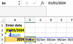
I copied your formula and only changed the , to ; as my Excel uses semicolons and not commas. I did not change anything else. I pasted the formula in cell A3 and get a #Value error. So I tried to trace the error and as far as I can see it points to cell B4. I have attached a screenshot of the trace and also of the value of B4 which is formatted to show a shorter date/month.

Any ideas?

R.
 

Attachments

  • Screenshot 2023-12-06 at 17.30.08.png
    Screenshot 2023-12-06 at 17.30.08.png
    44.2 KB · Views: 4
  • Screenshot 2023-12-06 at 17.33.02.png
    Screenshot 2023-12-06 at 17.33.02.png
    125.5 KB · Views: 5
Upvote 0
Im sorry i forgot to change the argument for the CELL function, if your excel is in english it should be "filename" not "nombrearchivo"

Here is the bb code again with the correction. Let me know if it works:

Goto.xlsx
ABCDEFGHIJKLM
1
204/01/2024
3Go to…
4202401/01/202402/01/202403/01/202404/01/202405/01/202406/01/202407/01/202408/01/202409/01/202410/01/202411/01/202412/01/2024
5
6
7
8
9
10
11202501/01/202502/01/202503/01/202504/01/202505/01/202506/01/202507/01/202508/01/202509/01/202510/01/202511/01/202512/01/2025
12
13
14
15
16
17
18202601/01/202602/01/202603/01/202604/01/202605/01/202606/01/202607/01/202608/01/202609/01/202610/01/202611/01/202612/01/2026
19
20
21
22
23
24
25
26
Sheet1 (2)
Cell Formulas
RangeFormula
A3A3=HYPERLINK(SUBSTITUTE("["&RIGHT(CELL("filename"),LEN(CELL("filename"))-FIND("[",CELL("filename"))),"]","]'")&"'!"&ADDRESS(MAX(ROW($B$4:$NC$18)*($B$4:$NC$18=A2)),MAX(COLUMN($B$4:$NC$18)*($B$4:$NC$18=A2))),"Go to…")
 
Upvote 0
Hi again - fast reply:)

Same result unfortunately. I tried entering 30/08/24 and 30/08/2024 in cell A2.
I also noticed that the formula somehow only covers years 2024 and 2025, but not 2026. Maybe this can be changed in your formula if we get it to work or is there a problem with how big a range (B4:NC18) can be put in this particular formula?

Please see attached.
 

Attachments

  • Screenshot 2023-12-06 at 17.59.53.png
    Screenshot 2023-12-06 at 17.59.53.png
    124.3 KB · Views: 3
Upvote 0
Just some further information. I tried setting the regional settings on my Mac to United States and copied your formula with "filename" and didn't change the commas (that are used as formula separators in Excel US version). The result was the same value error..
 
Upvote 0
Ohhh I think I can guess what the problem is why it wont work. Are you using the web application?
 
Upvote 0
just found this on Google:
Since 2016, Microsoft Excel has run in an App Sandbox on macOS. This means that a HYPERLINK function which points to a local path, like HYPERLINK("/Users/me/Desktop/example. pdf") , won't work.
 
Upvote 0

Forum statistics

Threads
1,215,988
Messages
6,128,146
Members
449,427
Latest member
jahaynes

We've detected that you are using an adblocker.

We have a great community of people providing Excel help here, but the hosting costs are enormous. You can help keep this site running by allowing ads on MrExcel.com.
Allow Ads at MrExcel

Which adblocker are you using?

Disable AdBlock

Follow these easy steps to disable AdBlock

1)Click on the icon in the browser’s toolbar.
2)Click on the icon in the browser’s toolbar.
2)Click on the "Pause on this site" option.
Go back

Disable AdBlock Plus

Follow these easy steps to disable AdBlock Plus

1)Click on the icon in the browser’s toolbar.
2)Click on the toggle to disable it for "mrexcel.com".
Go back

Disable uBlock Origin

Follow these easy steps to disable uBlock Origin

1)Click on the icon in the browser’s toolbar.
2)Click on the "Power" button.
3)Click on the "Refresh" button.
Go back

Disable uBlock

Follow these easy steps to disable uBlock

1)Click on the icon in the browser’s toolbar.
2)Click on the "Power" button.
3)Click on the "Refresh" button.
Go back
Back
Top