Help with IF formula

[southcity]

Hi guys,
I really need help to set up a logical solution to this.
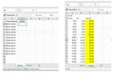
In 'Value' column I want to have a value based on time interval. If a time interval in a cell in Sheet 1 falls inside a time interval in Sheet 2 then take the values shown in Sheet 2, otherwise 40.
See image. THANKS FOR HELPING

 

[Legacy 143009]

Could you please provide some sample results for Sheet1 Column B?
There are several 09:51-10:00 in column A and there are several results fall into this range in Sheet2.

 

[Leo Skywalker]

In fact,

There are only 3 intervales in Sheet1:
9:51-10:00
16:04-16:09
9:12-9:27

From these, only 9:12-9:27 overlaps 9:10-9:25 in Sheet2, value 105.63, what about the time between 9:25-9:27??? the value does not apply anymore.

 

[fjns]

Hi, see the linked file for a possible solution...

The formula used in the table:
B2: =IF(INDEX(Sheet2!B:B,MATCH((100*LEFT(A2,2)+MID(A2,4,2))/100,Sheet2!A:A))>=(100*MID(A2,7,2)+RIGHT(A2,2))/100,INDEX(Sheet2!C:C,MATCH((100*LEFT(A2,2)+MID(A2,4,2))/100,Sheet2!A:A)),40) (Range: B2:B18)

ExcelFraga.xlsx

 

[southcity]

Hi, see the linked file for a possible solution...

The formula used in the table:
B2: =IF(INDEX(Sheet2!B:B,MATCH((100*LEFT(A2,2)+MID(A2,4,2))/100,Sheet2!A:A))>=(100*MID(A2,7,2)+RIGHT(A2,2))/100,INDEX(Sheet2!C:C,MATCH((100*LEFT(A2,2)+MID(A2,4,2))/100,Sheet2!A:A)),40) (Range: B2:B18)

ExcelFraga.xlsx

Wow! Thanks a lot. You already spared my tons of time, otherwise I would manually do this for 3000 rows ^_^
I have one more question though. Is there possible to change the formula to give me a value if the time interval falls at least 75% within any time value in Sheet2?
For example:
If I need the value for time interval 16:56-17:09 (Sheet1) and the available value for approx. that time is 16,50 to 17,05 with belonging value (Sheet2). Is it possible to make the formula to take that value if the time range falls in at least 75%? Or is it too advance? ^_^
Btw I added more values at sheet2 because apparently I forget to type in all the values.

Best regards,

 

[fjns]

Hi, the new table with six additional columns is ready. These six columns help you check. If you don't need them, you can delete them from the table.

The new formula used in the table:
B2: =LET(s1fh,LEFT(A2,2),s1fm,MID(A2,4,2),s1th,MID(A2,7,2),s1tm,RIGHT(A2,2),ix,MATCH((100*s1fh+s1fm)/100,Sheet2!A:A),s2f1,INDEX(Sheet2!A:A,ix),s2t1,INDEX(Sheet2!B:B,ix),s2v1,INDEX(Sheet2!C:C,ix),s2f1h,INT(s2f1),s2f1m,100*(s2f1-s2f1h),s2t1h,INT(s2t1),s2t1m,100*(s2t1-s2t1h),s2f2,INDEX(Sheet2!A:A,ix+1),s2t2,INDEX(Sheet2!B:B,ix+1),s2t2u,MIN((100*s1th+s1tm)/100,s2t2),s2v2,INDEX(Sheet2!C:C,ix+1),s2f2h,INT(s2f2),s2f2m,100*(s2f2-s2f2h),s2t2h,INT(s2t2),s2t2m,100*(s2t2-s2t2h),s2t2uh,INT(s2t2u),s2t2um,100*(s2t2u-s2t2uh),IFERROR(IF(s2t1>=(100*s1th+s1tm)/100,s2v1,IF(AND(s2t1>=(100*s1fh+s1fm)/100,((s2t1h-s1fh)*60+s2t1m-s1fm)/((s2t1h-s2f1h)*60+s2t1m-s2f1m)>=75/100),s2v1,IF(AND(s2f2=0,s2t2=0),40,IF(AND(s2t2u>=(100*s2f2h+s2f2m)/100,((s2t2uh-s2f2h)*60+s2t2um-s2f2m)/((s2t2h-s2f2h)*60+s2t2m-s2f2m)>=75/100),s2v2,40)))),40)) (Range: B2:B2977)

ExcelFragaNew.xlsx

 

[southcity]

Hi, the new table with six additional columns is ready. These six columns help you check. If you don't need them, you can delete them from the table.

The new formula used in the table:
B2: =LET(s1fh,LEFT(A2,2),s1fm,MID(A2,4,2),s1th,MID(A2,7,2),s1tm,RIGHT(A2,2),ix,MATCH((100*s1fh+s1fm)/100,Sheet2!A:A),s2f1,INDEX(Sheet2!A:A,ix),s2t1,INDEX(Sheet2!B:B,ix),s2v1,INDEX(Sheet2!C:C,ix),s2f1h,INT(s2f1),s2f1m,100*(s2f1-s2f1h),s2t1h,INT(s2t1),s2t1m,100*(s2t1-s2t1h),s2f2,INDEX(Sheet2!A:A,ix+1),s2t2,INDEX(Sheet2!B:B,ix+1),s2t2u,MIN((100*s1th+s1tm)/100,s2t2),s2v2,INDEX(Sheet2!C:C,ix+1),s2f2h,INT(s2f2),s2f2m,100*(s2f2-s2f2h),s2t2h,INT(s2t2),s2t2m,100*(s2t2-s2t2h),s2t2uh,INT(s2t2u),s2t2um,100*(s2t2u-s2t2uh),IFERROR(IF(s2t1>=(100*s1th+s1tm)/100,s2v1,IF(AND(s2t1>=(100*s1fh+s1fm)/100,((s2t1h-s1fh)*60+s2t1m-s1fm)/((s2t1h-s2f1h)*60+s2t1m-s2f1m)>=75/100),s2v1,IF(AND(s2f2=0,s2t2=0),40,IF(AND(s2t2u>=(100*s2f2h+s2f2m)/100,((s2t2uh-s2f2h)*60+s2t2um-s2f2m)/((s2t2h-s2f2h)*60+s2t2m-s2f2m)>=75/100),s2v2,40)))),40)) (Range: B2:B2977)

ExcelFragaNew.xlsx

It seems to be an error:

 

[fjns]

The error is only visible on Google Drive, because Google Drive does not know the LET function.

 

[southcity]

The error is only visible on Google Drive, because Google Drive does not know the LET function.

THANKS A LOT! You saved me tons of time and my colleagues now think that I am an excel wizard :P

 

[fjns]

THANKS A LOT! You saved me tons of time and my colleagues now think that I am an excel wizard :P

Hi, I am very glad that the new table is working well.
If I have enough knowledge, I am happy to help at any time.