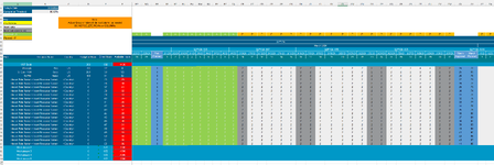
I have a spread that is used for labor tracking. Assume every cell represents a day. I want to be able to specify a percentage of labor completed against the plan, every month. So, if there were 80 hours available and someone worked 8 hours a day. The planned hours would be consumed after 10 days. I want to use conditional formatting to change the color of the appropriate cells based on a percentage, i.e., if the percentage is 80%, then every every cell >= 64 hours, i.e. ,days 8, 9, and 10 should have the conditional formatting rule apply. I don't know how to write a formula that will calculate the sum of cell1 against the value of cell 1, then the sum of (cell1 + cell2) against the value of cell 2, the sum of (cell1 + cell2 + cell3) against the value of cell3. In the image that I have uploaded, I would like to set his formula for the range BS17 to CW17. I apologize that I cannot upload a snippet using the XLBB add-in at the moment. I am getting an error message that it cannot run/is not allowed in protected mode.
-
If you would like to post, please check out the MrExcel Message Board FAQ and register here. If you forgot your password, you can reset your password.
You are using an out of date browser. It may not display this or other websites correctly.
You should upgrade or use an alternative browser.
You should upgrade or use an alternative browser.
How do you calculate a conditional sum for conditional formatting?
- Thread starter mkrass
- Start date
Excel Facts
Create a chart in one keystroke
Select the data and press Alt+F1 to insert a default chart. You can change the default chart to any chart type
awoohaw
Well-known Member
- Joined
- Mar 23, 2022
- Messages
- 4,568
- Office Version
- 365
- Platform
- Windows
- Web
in lieu of xl2bb you can post a table. just copy a range of cells and paste into the post. Your image is hard to read and has a lot of data. Just a few rows. And please show expected results.
in your scenario, why is day 8 supposed to be highlighted? 8x8 =64, so that has been met.
in your scenario, why is day 8 supposed to be highlighted? 8x8 =64, so that has been met.
Upvote
0
StephenCrump
MrExcel MVP
- Joined
- Sep 18, 2013
- Messages
- 5,402
- Office Version
- 365
- Platform
- Windows
In addition to @awoohaw's questions, perhaps you could also explain, is this question any different (apart from layout) to the similar question solved here:
Highlight cell when a percentage amount has been met.
Highlight cell when a percentage amount has been met.
Upvote
0
Peter_SSs
MrExcel MVP, Moderator
- Joined
- May 28, 2005
- Messages
- 63,880
- Office Version
- 365
- Platform
- Windows
I agree with @StephenCrump that this looks very similar to the thread he linked to. But in relation to this ..

 www.mrexcel.com
.. look through the suggestions in this thread:I cannot upload a snippet using the XLBB add-in at the moment. I am getting an error message that it cannot run/is not allowed in protected mode.
XL2BB Icons greyed out
Hi Team, i am unable to copy the data throught Xl2bb as buttom got disable please see the screen shot can anyone hlep me this. Regards Sanjeev
Upvote
0
Thank you all for your responses. I have been able to get XL2BB installed, so hopefully, the attached sample will help.In addition to @awoohaw's questions, perhaps you could also explain, is this question any different (apart from layout) to the similar question solved here:
Highlight cell when a percentage amount has been met.
")
In response to the question what is different from my post from last week, I would like to understand the syntax change if I need to use/calculate different time blocks, and exclude a summary cell. Also, with the attached sample, the previous solution, that did work, isn't working, and I would like to understand what I did wrong. So, from the included sample. If 0.81 is the percentage, I would expect that cells M3 and cells O3:X3 would be highlighted. The conditional calculation is if the sum is greater than or equal to the sum of the total labor hours and the percentage.
| Percentage test.xlsx | ||||||||||||||||||||||||||
|---|---|---|---|---|---|---|---|---|---|---|---|---|---|---|---|---|---|---|---|---|---|---|---|---|---|---|
| B | C | D | E | F | G | H | I | J | K | L | M | N | O | P | Q | R | S | T | U | V | W | X | Y | |||
| 1 | Time Block 1 | Block 1 Total | Time Block 2 | Block 2 Total | ||||||||||||||||||||||
| 2 | Budgeted Hours | 1/1/24 | 1/2/24 | 1/3/24 | 1/4/24 | 1/5/24 | 1/6/24 | 1/7/24 | 1/8/24 | 1/9/24 | 1/10/24 | 1/1/12024 | 1/12/24 | 1/33/2024 | 1/14/24 | 1/15/24 | 1/16/24 | 1/17/24 | 1/18/24 | 1/19/24 | 1/20/24 | |||||
| 3 | 160 | 8 | 8 | 8 | 8 | 8 | 8 | 8 | 8 | 8 | 8 | 80 | 8 | 8 | 8 | 8 | 8 | 8 | 8 | 8 | 8 | 8 | 80 | |||
| 4 | ||||||||||||||||||||||||||
| 5 | 0.85 | |||||||||||||||||||||||||
Sheet1 | ||||||||||||||||||||||||||
| Cell Formulas | ||
|---|---|---|
| Range | Formula | |
| N3,Y3 | N3 | =SUM(D3:M3) |
| Cells with Conditional Formatting | ||||
|---|---|---|---|---|
| Cell | Condition | Cell Format | Stop If True | |
| X3 | Expression | =SUM($D3:D3) >= $B3*$B5 | text | NO |
| W3 | Expression | =SUM($D3:D3) >= $B3*$B5 | text | NO |
| U3 | Expression | =SUM($D3:D3) >= $B3*$B5 | text | NO |
| T3 | Expression | =SUM($D3:D3) >= $B3*$B5 | text | NO |
| S3 | Expression | =SUM($D3:D3) >= $B3*$B5 | text | NO |
| R3 | Expression | =SUM($D3:D3) >= $B3*$B5 | text | NO |
| Q3 | Expression | =SUM($D3:D3) >= $B3*$B5 | text | NO |
| P3 | Expression | =SUM($D3:D3) >= $B3*$B5 | text | NO |
| O3 | Expression | =SUM($D3:D3) >= $B3*$B5 | text | NO |
| U5:W5 | Cell Value | >="($B$3*$B$5)" | text | NO |
| V3 | Expression | =SUM($D3:D3) >= $B3*$B5 | text | NO |
| M3 | Expression | =SUM($D3:D3) >= $B3*$B5 | text | NO |
| L3 | Expression | =SUM($D3:D3) >= $B3*$B5 | text | NO |
| J3 | Expression | =SUM($D3:D3) >= $B3*$B5 | text | NO |
| I3 | Expression | =SUM($D3:D3) >= $B3*$B5 | text | NO |
| H3 | Expression | =SUM($D3:D3) >= $B3*$B5 | text | NO |
| G3 | Expression | =SUM($D3:D3) >= $B3*$B5 | text | NO |
| F3 | Expression | =SUM($D3:D3) >= $B3*$B5 | text | NO |
| E3 | Expression | =SUM($D3:D3) >= $B3*$B5 | text | NO |
| D3 | Expression | =SUM($D3:D3) >= $B3*$B5 | text | NO |
| J5:L5 | Cell Value | >="($B$3*$B$5)" | text | NO |
| K3 | Expression | =SUM($D3:D3)>=$B$3*$B$5 | text | NO |
Upvote
0
StephenCrump
MrExcel MVP
- Joined
- Sep 18, 2013
- Messages
- 5,402
- Office Version
- 365
- Platform
- Windows
Excellent!I have been able to get XL2BB installed ...
How about ...
| A | B | C | D | E | F | G | H | I | J | K | L | M | N | O | P | Q | R | S | T | U | V | W | X | Y | |||
|---|---|---|---|---|---|---|---|---|---|---|---|---|---|---|---|---|---|---|---|---|---|---|---|---|---|---|---|
| 1 | Time Block 1 | Block 1 | Time Block 2 | Block 2 | |||||||||||||||||||||||
| 2 | Budgeted Hours | 1 Jan 2024 | 2 Jan 2024 | 3 Jan 2024 | 4 Jan 2024 | 5 Jan 2024 | 6 Jan 2024 | 7 Jan 2024 | 8 Jan 2024 | 9 Jan 2024 | 10 Jan 2024 | Total | 11 Jan 2024 | 12 Jan 2024 | 13 Jan 2024 | 14 Jan 2024 | 15 Jan 2024 | 16 Jan 2024 | 17 Jan 2024 | 18 Jan 2024 | 19 Jan 2024 | 20 Jan 2024 | Total | ||||
| 3 | 160 | 8 | 8 | 8 | 8 | 8 | 8 | 8 | 8 | 8 | 8 | 80 | 8 | 8 | 8 | 8 | 8 | 8 | 8 | 8 | 8 | 8 | 80 | ||||
| 4 | 10 | 10 | 10 | 10 | 10 | 10 | 10 | 10 | 10 | 10 | 100 | 10 | 10 | 10 | 10 | 10 | 10 | 10 | 10 | 10 | 10 | 100 | |||||
| 5 | 0.6 | 9 | 9 | 9 | 9 | 9 | 9 | 9 | 9 | 9 | 9 | 90 | 9 | 9 | 9 | 9 | 9 | 9 | 9 | 9 | 9 | 9 | 90 | ||||
Sheet1 | |||||||||||||||||||||||||||
| Cell Formulas | ||
|---|---|---|
| Range | Formula | |
| N3:N5,Y3:Y5 | N3 | =SUM(D3:M3) |
| Cells with Conditional Formatting | ||||
|---|---|---|---|---|
| Cell | Condition | Cell Format | Stop If True | |
| D3:Y5 | Expression | =SUMPRODUCT($D3:D3,--ISNUMBER($D$2:D$2))>=$B$3*$B$5 | text | NO |
Upvote
0
In addition to @awoohaw's questions, perhaps you could also explain, is this question any different (apart from layout) to the similar question solved here:
Highlight cell when a percentage amount has been met.
Stephen, Thank you. I applied the formula to teh same sample spreadsheet I uploaded, and no conditional formattong was applied, see enclosedExcellent!
How about ...
A B C D E F G H I J K L M N O P Q R S T U V W X Y 1 Time Block 1 Block 1 Time Block 2 Block 2 2 Budgeted Hours 1 Jan 2024 2 Jan 2024 3 Jan 2024 4 Jan 2024 5 Jan 2024 6 Jan 2024 7 Jan 2024 8 Jan 2024 9 Jan 2024 10 Jan 2024 Total 11 Jan 2024 12 Jan 2024 13 Jan 2024 14 Jan 2024 15 Jan 2024 16 Jan 2024 17 Jan 2024 18 Jan 2024 19 Jan 2024 20 Jan 2024 Total 3 160 8 8 8 8 8 8 8 8 8 8 80 8 8 8 8 8 8 8 8 8 8 80 4 10 10 10 10 10 10 10 10 10 10 100 10 10 10 10 10 10 10 10 10 10 100 5 0.6 9 9 9 9 9 9 9 9 9 9 90 9 9 9 9 9 9 9 9 9 9 90
Cell Formulas Range Formula N3:N5,Y3:Y5 N3 =SUM(D3:M3)
Cells with Conditional Formatting Cell Condition Cell Format Stop If True D3:Y5 Expression =SUMPRODUCT($D3:D3,--ISNUMBER($D$2:D$2))>=$B$3*$B$5 text NO
| Percentage test.xlsx | |||||||||||||||||||||||||||
|---|---|---|---|---|---|---|---|---|---|---|---|---|---|---|---|---|---|---|---|---|---|---|---|---|---|---|---|
| A | B | C | D | E | F | G | H | I | J | K | L | M | N | O | P | Q | R | S | T | U | V | W | X | Y | |||
| 1 | Time Block 1 | Block 1 Total | Time Block 2 | Block 2 Total | |||||||||||||||||||||||
| 2 | Budgeted Hours | 1/1/24 | 1/2/24 | 1/3/24 | 1/4/24 | 1/5/24 | 1/6/24 | 1/7/24 | 1/8/24 | 1/9/24 | 1/10/24 | 1/1/12024 | 1/12/24 | 1/33/2024 | 1/14/24 | 1/15/24 | 1/16/24 | 1/17/24 | 1/18/24 | 1/19/24 | 1/20/24 | ||||||
| 3 | 160 | 8 | 8 | 8 | 8 | 8 | 8 | 8 | 8 | 8 | 8 | 80 | 8 | 8 | 8 | 8 | 8 | 8 | 8 | 8 | 8 | 8 | 80 | ||||
| 4 | |||||||||||||||||||||||||||
| 5 | 0.40 | ||||||||||||||||||||||||||
Sheet1 | |||||||||||||||||||||||||||
| Cell Formulas | ||
|---|---|---|
| Range | Formula | |
| N3,Y3 | N3 | =SUM(D3:M3) |
| Cells with Conditional Formatting | ||||
|---|---|---|---|---|
| Cell | Condition | Cell Format | Stop If True | |
| X3 | Expression | =SUMPRODUCT($D3:D3,--ISNUMBER($D$2:D$2))>=$B$3*$B$5 | text | NO |
| W3 | Expression | =SUMPRODUCT($D3:D3,--ISNUMBER($D$2:D$2))>=$B$3*$B$5 | text | NO |
| U3 | Expression | =SUMPRODUCT($D3:D3,--ISNUMBER($D$2:D$2))>=$B$3*$B$5 | text | NO |
| T3 | Expression | =SUMPRODUCT($D3:D3,--ISNUMBER($D$2:D$2))>=$B$3*$B$5 | text | NO |
| S3 | Expression | =SUMPRODUCT($D3:D3,--ISNUMBER($D$2:D$2))>=$B$3*$B$5 | text | NO |
| R3 | Expression | =SUMPRODUCT($D3:D3,--ISNUMBER($D$2:D$2))>=$B$3*$B$5 | text | NO |
| Q3 | Expression | =SUMPRODUCT($D3:D3,--ISNUMBER($D$2:D$2))>=$B$3*$B$5 | text | NO |
| P3 | Expression | =SUMPRODUCT($D3:D3,--ISNUMBER($D$2:D$2))>=$B$3*$B$5 | text | NO |
| O3 | Expression | =SUMPRODUCT($D3:D3,--ISNUMBER($D$2:D$2))>=$B$3*$B$5 | text | NO |
| U5:W5 | Cell Value | >="($B$3*$B$5)" | text | NO |
| V3 | Expression | =SUMPRODUCT($D3:D3,--ISNUMBER($D$2:D$2))>=$B$3*$B$5 | text | NO |
| M3 | Expression | =SUMPRODUCT($D3:D3,--ISNUMBER($D$2:D$2))>=$B$3*$B$5 | text | NO |
| L3 | Expression | =SUMPRODUCT($D3:D3,--ISNUMBER($D$2:D$2))>=$B$3*$B$5 | text | NO |
| J3 | Expression | =SUMPRODUCT($D3:D3,--ISNUMBER($D$2:D$2))>=$B$3*$B$5 | text | NO |
| I3 | Expression | =SUMPRODUCT($D3:D3,--ISNUMBER($D$2:D$2))>=$B$3*$B$5 | text | NO |
| H3 | Expression | =SUMPRODUCT($D3:D3,--ISNUMBER($D$2:D$2))>=$B$3*$B$5 | text | NO |
| G3 | Expression | =SUMPRODUCT($D3:D3,--ISNUMBER($D$2:D$2))>=$B$3*$B$5 | text | NO |
| F3 | Expression | =SUMPRODUCT($D3:D3,--ISNUMBER($D$2:D$2))>=$B$3*$B$5 | text | NO |
| E3 | Expression | =SUMPRODUCT($D3:D3,--ISNUMBER($D$2:D$2))>=$B$3*$B$5 | text | NO |
| D3 | Expression | =SUMPRODUCT($D3:D3,--ISNUMBER($D$2:D$2))>=$B$3*$B$5 | text | NO |
| J5:L5 | Cell Value | >="($B$3*$B$5)" | text | NO |
| K3 | Expression | =SUMPRODUCT($D3:D3,--ISNUMBER($D$2:D$2))>=$B$3*$B$5 | text | NO |
Upvote
0
Peter_SSs
MrExcel MVP, Moderator
- Joined
- May 28, 2005
- Messages
- 63,880
- Office Version
- 365
- Platform
- Windows
I applied the formula to teh same sample spreadsheet I uploaded
- Not correctly. You have applied the CF formula individually to lots of separate cells. You need to select thee whole row of cells and apply the CF formula once. However, I don't think that formula will quite do what you want given this from your earlier example.
I would expect that cells M3 and cells O3:X3 would be highlighted. - Also, your sample sheet has dates that are not actually dates in some of the row 2 cells (eg O2 and Q2) so that will mess things up too.
This is my suggestion. Delete any existing CF in row 3 then select from D3:Y3 (or further to the right if there are more dates) and then apply this CF
| mkrass.xlsm | |||||||||||||||||||||||||||
|---|---|---|---|---|---|---|---|---|---|---|---|---|---|---|---|---|---|---|---|---|---|---|---|---|---|---|---|
| A | B | C | D | E | F | G | H | I | J | K | L | M | N | O | P | Q | R | S | T | U | V | W | X | Y | |||
| 1 | Time Block 1 | Block 1 Total | Time Block 2 | Block 2 Total | |||||||||||||||||||||||
| 2 | Budgeted Hours | 1/1/2024 | 2/1/2024 | 3/1/2024 | 4/1/2024 | 5/1/2024 | 6/1/2024 | 7/1/2024 | 8/1/2024 | 9/1/2024 | 10/1/2024 | 11/1/2024 | 12/1/2024 | 13/1/2024 | 14/1/2024 | 15/1/2024 | 16/1/2024 | 17/1/2024 | 18/1/2024 | 19/1/2024 | 20/1/2024 | ||||||
| 3 | 160 | 8 | 8 | 8 | 8 | 8 | 8 | 8 | 8 | 8 | 8 | 80 | 8 | 8 | 8 | 8 | 8 | 8 | 8 | 8 | 8 | 8 | 80 | ||||
| 4 | |||||||||||||||||||||||||||
| 5 | 0.4 | ||||||||||||||||||||||||||
CF (3) | |||||||||||||||||||||||||||
| Cell Formulas | ||
|---|---|---|
| Range | Formula | |
| N3,Y3 | N3 | =SUM(D3:M3) |
| Cells with Conditional Formatting | ||||
|---|---|---|---|---|
| Cell | Condition | Cell Format | Stop If True | |
| D3:Y3 | Expression | =AND(ISNUMBER(D$2),SUMIFS($D3:D3,$D$2:D$2,"<>*Total")>=$B$3*$B$5) | text | NO |
Upvote
0
Peter, Thank you. This is now working. I can see the CF rule being applied.
- Not correctly. You have applied the CF formula individually to lots of separate cells. You need to select thee whole row of cells and apply the CF formula once. However, I don't think that formula will quite do what you want given this from your earlier example.
- Also, your sample sheet has dates that are not actually dates in some of the row 2 cells (eg O2 and Q2) so that will mess things up too.
This is my suggestion. Delete any existing CF in row 3 then select from D3:Y3 (or further to the right if there are more dates) and then apply this CF
mkrass.xlsm
A B C D E F G H I J K L M N O P Q R S T U V W X Y 1 Time Block 1 Block 1 Total Time Block 2 Block 2 Total 2 Budgeted Hours 1/1/2024 2/1/2024 3/1/2024 4/1/2024 5/1/2024 6/1/2024 7/1/2024 8/1/2024 9/1/2024 10/1/2024 11/1/2024 12/1/2024 13/1/2024 14/1/2024 15/1/2024 16/1/2024 17/1/2024 18/1/2024 19/1/2024 20/1/2024 3 160 8 8 8 8 8 8 8 8 8 8 80 8 8 8 8 8 8 8 8 8 8 80 4 5 0.4
Cell Formulas Range Formula N3,Y3 N3 =SUM(D3:M3)
Cells with Conditional Formatting Cell Condition Cell Format Stop If True D3:Y3 Expression =AND(ISNUMBER(D$2),SUMIFS($D3:D3,$D$2:D$2,"<>*Total")>=$B$3*$B$5) text NO
(I did learn something from your post. I didn't realize you can select a range and apply the CF rule once for all - thank you for that).
But, it appears to include the value of N3 and Y3. Am I reading that correctly? How can the N3 and Y3 column values be excluded from the calculation?
Upvote
0
Peter_SSs
MrExcel MVP, Moderator
- Joined
- May 28, 2005
- Messages
- 63,880
- Office Version
- 365
- Platform
- Windows
Sorry, I missed the fact that those total columns have merged cells in rows 1 & 2. As it happens that makes the formula marginally simpler.But, it appears to include the value of N3 and Y3. Am I reading that correctly? How can the N3 and Y3 column values be excluded from the calculation?
| mkrass.xlsm | |||||||||||||||||||||||||||
|---|---|---|---|---|---|---|---|---|---|---|---|---|---|---|---|---|---|---|---|---|---|---|---|---|---|---|---|
| A | B | C | D | E | F | G | H | I | J | K | L | M | N | O | P | Q | R | S | T | U | V | W | X | Y | |||
| 1 | Time Block 1 | Block 1 Total | Time Block 2 | Block 2 Total | |||||||||||||||||||||||
| 2 | Budgeted Hours | 1/1/2024 | 2/1/2024 | 3/1/2024 | 4/1/2024 | 5/1/2024 | 6/1/2024 | 7/1/2024 | 8/1/2024 | 9/1/2024 | 10/1/2024 | 11/1/2024 | 12/1/2024 | 13/1/2024 | 14/1/2024 | 15/1/2024 | 16/1/2024 | 17/1/2024 | 18/1/2024 | 19/1/2024 | 20/1/2024 | ||||||
| 3 | 160 | 8 | 8 | 8 | 8 | 8 | 8 | 8 | 8 | 8 | 8 | 80 | 8 | 8 | 8 | 8 | 8 | 8 | 8 | 8 | 8 | 8 | 80 | ||||
| 4 | |||||||||||||||||||||||||||
| 5 | 0.7 | ||||||||||||||||||||||||||
CF (3) | |||||||||||||||||||||||||||
| Cell Formulas | ||
|---|---|---|
| Range | Formula | |
| N3,Y3 | N3 | =SUM(D3:M3) |
| Cells with Conditional Formatting | ||||
|---|---|---|---|---|
| Cell | Condition | Cell Format | Stop If True | |
| D3:Y3 | Expression | =AND(ISNUMBER(D$2),SUMIFS($D3:D3,$D$2:D$2,"<>")>=$B$3*$B$5) | text | NO |
Upvote
0
Solution
Similar threads
- Replies
- 8
- Views
- 407
- Replies
- 3
- Views
- 374
- Replies
- 21
- Views
- 1K
- Replies
- 3
- Views
- 465


