Please note: I have posted this question on another website a few days ago and have not received any answers to it. I am hoping on of you kind folks here might know the answer.
I am creating time cards and need 260 of them. I want to simply create one, and then copy paste, duplicating each copy/paste until I have 260. The problem is, formula references are taking account for cells in between each other. In other words, If I have a formula in A1 and A6, and data in the cells in between that also needs to be copied.
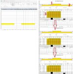
I have attached the sample workbook and a photo showing what I want to copy and where.
I need the formulas I copy down without loosing reference (staying sequentially correct) despite other rows in between have data. As it stands now, when I try to paste formula, it calculates all the lines in between the yellow boxes so numerically, it's not referencing the correct cell in the different sheet.
I found this formula listed on another website post and wonder if this would work for what I need to do: =INDIRECT("sheet1!B"& ROW(A5)/5)
I am using VLOOKUP and I tried this code:
=IFERROR(VLOOKUP(B6,Sunday!$A6:$K6,6,FALSE),"")
However I can't figure out how to combine INDIRECT with the VLOOKUP. In my original (real workbook) there are 29 rows between B6 and B35. Same between G5 and G34, and also between D12 and D41.
Can someone help me figure out a way to be able to copy the whole timesheet and duplicate it again and again? I need 260 of them
Also posted here How to duplicate a block of cells that contain formulas without losing reference?
here How to duplicate a block of cells that contain formulas without losing reference?
here How to duplicate a block of cells without losing formula references
I am creating time cards and need 260 of them. I want to simply create one, and then copy paste, duplicating each copy/paste until I have 260. The problem is, formula references are taking account for cells in between each other. In other words, If I have a formula in A1 and A6, and data in the cells in between that also needs to be copied.
I have attached the sample workbook and a photo showing what I want to copy and where.
I need the formulas I copy down without loosing reference (staying sequentially correct) despite other rows in between have data. As it stands now, when I try to paste formula, it calculates all the lines in between the yellow boxes so numerically, it's not referencing the correct cell in the different sheet.
I found this formula listed on another website post and wonder if this would work for what I need to do: =INDIRECT("sheet1!B"& ROW(A5)/5)
I am using VLOOKUP and I tried this code:
=IFERROR(VLOOKUP(B6,Sunday!$A6:$K6,6,FALSE),"")
However I can't figure out how to combine INDIRECT with the VLOOKUP. In my original (real workbook) there are 29 rows between B6 and B35. Same between G5 and G34, and also between D12 and D41.
Can someone help me figure out a way to be able to copy the whole timesheet and duplicate it again and again? I need 260 of them
| Sample Book.xlsx | |||
|---|---|---|---|
| E | |||
| 45 | |||
Timesheet | |||
| Sample Book.xlsx | ||||||||||
|---|---|---|---|---|---|---|---|---|---|---|
| C | D | E | F | G | H | I | J | |||
| 29 | 22:00 | 23:00 | 24:00 | 25:00 | 26:00 | 27:00 | 28:00 | 29:00 | ||
Raw Entries | ||||||||||
Also posted here How to duplicate a block of cells that contain formulas without losing reference?
here How to duplicate a block of cells that contain formulas without losing reference?
here How to duplicate a block of cells without losing formula references
Attachments
Last edited by a moderator:


