How to extract minimum value and show in another cell based on drop down list

[munchems]

Hello,

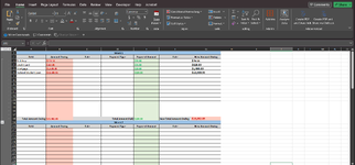
I'm a beginner excel user and I am trying to take the minimum value from the "New Amount Owing" column in Week 1 and show it in the "Amount Owing" column Week 2 based on the drop down list selection in the "Debt" column of Week 2. I've tried nesting IF and MINIF but haven't been sucsessful. TIA!

 

[Legacy 143009]

Hello,

What is the condition? Greater than debt or smaller than debt?

 

[munchems]

Hello,

What is the condition? Greater than debt or smaller than debt?

What I want to happen is for the Amount Owing under Week 2 to show the latest amount owing based on the list item chosen in the Debt column (List Items: Toll Hwy, Mortgage, Credit Card, Federal Student Loan) of Week 2 and to continue to update to the new amount owing based on the list item chosen. There will be subsequent weeks added to this sheet as well. I'm really sorry if this isn't clear enough. I'm having a hard time articulating my goal.

 

[munchems]

Hello,

What is the condition? Greater than debt or smaller than debt?

I came up with this formula

=IF(A22="407 ETR", MINIFS(G3:G17, A3:A17, "=407 ETR"), IF(A22="Rogers", MINIFS(G3:G17, A3:A17, "=Rogers"), IF(A22="Capital One", MINIFS(G3:G17, A3:A17, "=Capital One"), IF(A22="Provincial Student Loan", MINIFS(G3:G17, A3:A17, "=Provincial Student Loan"), IF(A22="Federal Student Loan", MINIFS(G3:G17, A3:A17, "=Federal Student Loan"), "")))))

however this doesn't take into acocunt that there will be new amount owing values in the G column under Week 2 as this is only taking data from G column in Week 1

 

[munchems]

Hello,

What is the condition? Greater than debt or smaller than debt?

My apologies this is the formula I meant to post:

=IF(A21:A35="Toll Hwy", MINIFS(G3:G17, A3:A17, "=Toll Hwy"), IF(A21:A35="Credit Card", MINIFS(G3:G17, A3:A17, "=Credit Card"), IF(A21:A35="Mortgage", MINIFS(G3:G17, A3:A17, "=Mortgage"), IF(A21:A35="Federal Student Loan", MINIFS(G3:G17, A3:A17, "=Federal Student Loan"), ""))))

 

[munchems]

I was able to acheive my goal! The starting debt amounts are in B3:B6 and in B7 I used this formula:

=IF(A7="Toll Hwy", MINIFS($G$3:$G$6, $A$3:$A$6, "=Toll Hwy"), IF(A7="Mortgage", MINIFS($G$3:$G$6, $A$3:$A$6, "=Mortgage"), IF(A7="Credit Card", MINIFS($G$3:G6, $A$3:A6, "=Credit Card"), IF(A7="Federal Student Loan", MINIFS($G$3:G6, $A$3:A6, "=Federal Student Loan"),""))))

and used this formula in the rest of the B column:

=IF(A8="Toll Hwy", MINIFS($G$3:G7, $A$3:A7, "=Toll Hwy"), IF(A8="Mortgage", MINIFS($G$3:G7, $A$3:A7, "=Mortgage"), IF(A8="Credit Card", MINIFS($G$3:G7, $A$3:A7, "=Credit Card"), IF(A8="Federal Student Loan", MINIFS($G$3:G7, $A$3:A7, "=Federal Student Loan"),""))))

 

[Peter_SSs]

I was able to acheive my goal!

Great news, but do you need those huge formulas? Perhaps I have not understood your layout or requirements properly but in the mini sheet below I have your formulas in B7:B9 and a much simpler alternative suggestion in C7:C9 which so far produces the same results as yours. Could you use those column C formulas instead of the current column B formulas?

23 11 15.xlsm
	A	B	C	D	E	F	G
3	Toll Hwy	111.14			35.00		76.14
4	Credit Card	663.00			35.00		628.00
5	Mortgage	1,500.00			20.00		1,480.00
6	Federal Student Loan	13,608.55			100.00		13,508.55
7	Credit Card	628.00	628.00		20.00		608.00
8	Mortgage	1,480.00	1,480.00		60.00		1,420.00
9	Credit Card	608.00	608.00		20.00		588.00
Lowest values

Cell Formulas
Range	Formula
B7	B7	=IF(A7="Toll Hwy", MINIFS($G$3:$G$6, $A$3:$A$6, "=Toll Hwy"), IF(A7="Mortgage", MINIFS($G$3:$G$6, $A$3:$A$6, "=Mortgage"), IF(A7="Credit Card", MINIFS($G$3:G6, $A$3:A6, "=Credit Card"), IF(A7="Federal Student Loan", MINIFS($G$3:G6, $A$3:A6, "=Federal Student Loan"),""))))
C7:C9	C7	=AGGREGATE(15,6,G$3:G6/(A$3:A6=A7),1)
B8:B9	B8	=IF(A8="Toll Hwy", MINIFS($G$3:G7, $A$3:A7, "=Toll Hwy"), IF(A8="Mortgage", MINIFS($G$3:G7, $A$3:A7, "=Mortgage"), IF(A8="Credit Card", MINIFS($G$3:G7, $A$3:A7, "=Credit Card"), IF(A8="Federal Student Loan", MINIFS($G$3:G7, $A$3:A7, "=Federal Student Loan"),""))))
G3:G9	G3	=B3-E3

 

[munchems]

Great news, but do you need those huge formulas? Perhaps I have not understood your layout or requirements properly but in the mini sheet below I have your formulas in B7:B9 and a much simpler alternative suggestion in C7:C9 which so far produces the same results as yours. Could you use those column C formulas instead of the current column B formulas?

23 11 15.xlsm
	A	B	C	D	E	F	G
3	Toll Hwy	111.14			35.00		76.14
4	Credit Card	663.00			35.00		628.00
5	Mortgage	1,500.00			20.00		1,480.00
6	Federal Student Loan	13,608.55			100.00		13,508.55
7	Credit Card	628.00	628.00		20.00		608.00
8	Mortgage	1,480.00	1,480.00		60.00		1,420.00
9	Credit Card	608.00	608.00		20.00		588.00
Lowest values

Cell Formulas
Range	Formula
B7	B7	=IF(A7="Toll Hwy", MINIFS($G$3:$G$6, $A$3:$A$6, "=Toll Hwy"), IF(A7="Mortgage", MINIFS($G$3:$G$6, $A$3:$A$6, "=Mortgage"), IF(A7="Credit Card", MINIFS($G$3:G6, $A$3:A6, "=Credit Card"), IF(A7="Federal Student Loan", MINIFS($G$3:G6, $A$3:A6, "=Federal Student Loan"),""))))
C7:C9	C7	=AGGREGATE(15,6,G$3:G6/(A$3:A6=A7),1)
B8:B9	B8	=IF(A8="Toll Hwy", MINIFS($G$3:G7, $A$3:A7, "=Toll Hwy"), IF(A8="Mortgage", MINIFS($G$3:G7, $A$3:A7, "=Mortgage"), IF(A8="Credit Card", MINIFS($G$3:G7, $A$3:A7, "=Credit Card"), IF(A8="Federal Student Loan", MINIFS($G$3:G7, $A$3:A7, "=Federal Student Loan"),""))))
G3:G9	G3	=B3-E3

As a beginner user I didn't even know AGGREGATE existed or how it works. Thank you!

 

[Peter_SSs]

I didn't even know AGGREGATE existed or how it works. Thank you!

You're welcome, but to be honest, I probably should have stuck to MINIFS that you were using. Wouldn't this very simple version of that function do the job for you?

23 11 15.xlsm
	A	B	C	D	E	F	G
3	Toll Hwy	111.14			35.00		76.14
4	Credit Card	663.00			35.00		628.00
5	Mortgage	1,500.00			20.00		1,480.00
6	Federal Student Loan	13,608.55			100.00		13,508.55
7	Credit Card	628.00			20.00		608.00
8	Mortgage	1,480.00			60.00		1,420.00
9	Credit Card	608.00			20.00		588.00
Lowest values (2)

Cell Formulas
Range	Formula
B7:B9	B7	=MINIFS(G$3:G6,A$3:A6,A7)
G3:G9	G3	=B3-E3

 

[munchems]

You're welcome, but to be honest, I probably should have stuck to MINIFS that you were using. Wouldn't this very simple version of that function do the job for you?

23 11 15.xlsm
	A	B	C	D	E	F	G
3	Toll Hwy	111.14			35.00		76.14
4	Credit Card	663.00			35.00		628.00
5	Mortgage	1,500.00			20.00		1,480.00
6	Federal Student Loan	13,608.55			100.00		13,508.55
7	Credit Card	628.00			20.00		608.00
8	Mortgage	1,480.00			60.00		1,420.00
9	Credit Card	608.00			20.00		588.00
Lowest values (2)

Cell Formulas
Range	Formula
B7:B9	B7	=MINIFS(G$3:G6,A$3:A6,A7)
G3:G9	G3	=B3-E3

No, that was one of the first things I tried. The reason it doesn't work is because there's no condition on what drop down list selection is chosen in column A.

You're welcome, but to be honest, I probably should have stuck to MINIFS that you were using. Wouldn't this very simple version of that function do the job for you?

23 11 15.xlsm
	A	B	C	D	E	F	G
3	Toll Hwy	111.14			35.00		76.14
4	Credit Card	663.00			35.00		628.00
5	Mortgage	1,500.00			20.00		1,480.00
6	Federal Student Loan	13,608.55			100.00		13,508.55
7	Credit Card	628.00			20.00		608.00
8	Mortgage	1,480.00			60.00		1,420.00
9	Credit Card	608.00			20.00		588.00
Lowest values (2)

Cell Formulas
Range	Formula
B7:B9	B7	=MINIFS(G$3:G6,A$3:A6,A7)
G3:G9	G3	=B3-E3

Yeah so that's exactly what I ended up using after I had posted my solution. I think coming up with that long formula helped me to understand how I could shorten it into a single MINIFS formula. But now I understand the AGGREGATE function as well and I'm learning a lot!! Thanks again!